Least Square
Least Square. y = f ( x ). Motivation. Given data points, fit a function that is “ close ” to the points Local surface fitting to 3D points. y. P i = ( x i , y i ). x. Line Fitting. y - offsets minimization. y. P i = ( x i , y i ). x. Line Fitting.

Least Square
E N D
Presentation Transcript
y = f (x) Motivation • Given data points, fit a function that is “close” to the points • Local surface fitting to 3D points y Pi = (xi, yi) x
Line Fitting • y-offsets minimization y Pi = (xi, yi) x
Line Fitting • Find a liney = ax + bthat minimizes • E(a,b)is quadratic in the unknown parametersa, b • Another option would be, for example: • But – it is not differentiable, harder to minimize…
Line Fitting – LS minimization • To find optimal a, b we differentiate E(a, b): E(a, b) = (–2xi)[yi – (axi + b)] = 0 E(a, b) = (–2)[yi – (axi + b)] = 0
Line Fitting – LS minimization • We get two linear equations for a, b: (–2xi)[yi – (axi + b)] = 0 (–2)[yi – (axi + b)] = 0 [xiyi – axi2 – bxi] = 0 [yi – axi – b] = 0
Line Fitting – LS minimization • We get two linear equations for a, b: ( xi2) a + ( xi) b = xiyi ( xi)a + ( 1)b = yi
Line Fitting – LS minimization • Solve for a, b using e.g. Gauss elimination • Question: why the solution is the minimum for the error function? E(a, b) = [yi – (axi + b)]2
Fitting Polynomials • Decide on the degree of the polynomial, k • Want to fit f (x) = akxk + ak-1xk-1 + … + a1x+ a0 • Minimize: E(a0,a1, …,ak) = [yi – (akxik+ak-1xik-1+ …+a1xi+a0)]2 E(a0,…,ak) = (– 2xm)[yi – (akxik+ak-1xik-1+…+ a0)] = 0
Fitting Polynomials • We get a linear system of k+1 in k+1 variables
General Parametric Fitting • We can use this approach to fit any function f(x) • Specified by parameters a, b, c, … • The expression f(x) linearly depends on the parameters a, b, c, …
General Parametric Fitting • Want to fit function fabc…(x) to data points (xi, yi) • Define E(a,b,c,…) = [yi – fabc…(xi)]2 • Solve the linear system
General Parametric Fitting • It can even be some crazy function like • Or in general:
Solving Linear Systems in LS Sense • Let’s look at the problem a little differently: • We have data points (xi, yi) • We want the function f(x) to go through the points: i =1, …, n: yi = f(xi) • Strict interpolation is in general not possible • In polynomials: n+1 points define a unique interpolation polynomial of degree n. • So, if we have 1000 points and want a cubic polynomial, we probably won’t find it…
Solving Linear Systems in LS Sense • We have an over-determined linear system nk: f(x1) = 1f1(x1) + 2f2(x1) + … + kfk(x1) = y1 f(x2) = 1f1(x2) + 2f2(x2) + … + kfk(x2) = y2 … … … f(xn) = 1f1(xn) + 2f2(xn) + … + kfk(xn) = yn
Solving Linear Systems in LS Sense • In matrix form:
Solving Linear Systems in LS Sense • In matrix form: Av = y
Solving Linear Systems in LS Sense • More constrains than variables – no exact solutions generally exist • We want to find something that is an “approximate solution”:
Finding the LS Solution • v Rk • Av Rn • As we vary v, Av varies over the linear subspace of Rnspanned by the columns of A: Av = = 1 + 2 +…+ k 1 2 . . k A1 A2 Ak A1 A2 Ak
Av closest to y Finding the LS Solution • We want to find the closest Av to y: y Subspace spanned by columns of A Rn
Finding the LS Solution • The vector Av closest to y satisfies: (Av – y) {subspace of A’s columns} column Ai, <Ai, Av – y> = 0 i, AiT(Av – y) = 0 AT(Av – y) = 0 (ATA)v = ATy These are called the normal equations
Finding the LS Solution • We got a square symmetric system • (ATA)v = ATy • If A has full rank (the columns of A are linearly independent) then (ATA) is invertible. (kk)
Handle Based Editing Handles, they are free to move by user Model deforms when handles are places at target positions
General Idea • A visually pleasing deformed mesh should maintain • local parameterization (triangle shape) • local geometry information (local shape) • We decompose the global geometry into • coefficients of the Laplace operator • Laplacian coordinates (LCs)
Laplacian Coordinates • LC represent local geometry • Coefficients of Laplacian operator represent local parameterization or xi xj ...
Laplacian Editing • We solve new vertex positions with handle constraints • In general there is no solution • We use LS method to find optimal solution Solve x:
Shape Matching • We have two objects in correspondence • Want to find the rigid transformation that aligns them
Shape Matching • When the objects are aligned, the lengths of the connecting lines are small.
Shape Matching – Formalization • Align two point sets • Find a translation vector t and rotation matrix R so that:
Shape Matching – Solution • Turns out we can solve the translation and rotation separately. • Theorem: if (R, t) is the optimal transformation, then the points {pi} and {Rqi + t} have the same centers of mass.
Finding the Rotation R • To find the optimal R, we bring the centroids of both point sets to the origin: • We want to find R that minimizes
Finding the Rotation R • First we compute optimum linear transformation A that minimizes • We solve it in LS sense and build the systems = Q = q0 q1 … qn P = p0 p1 … pn A QT PT AT = 3x3
Finding the Rotation R • We can solve columns of AT = {a1, a2, a3} superlatively • By using LS method QQT AT = QPT A = (QQT)-1(QPT) QT = PT a1 a2 a3 3x1 3x3 3x3
Finding the Rotation R • Second we extract the pure rotation part R from A • We use singular value decomposition (SVD) • A = UWV • A = RS • R = UV, S = VTWV • Since U and V are orthogonal, therefore R does • S is a positive-semidefinite symetric matrix • Finally we compute translation t = p - Rq U, V: orthogonal matricesW: diagonal matrix
Reference • SVD • Numerical Recipes in C (section2.6) • http://www.nrbook.com/a/bookcpdf.php • A Tutorial on Principal Component Analysis • http://www.snl.salk.edu/~shlens/pub/notes/pca.pdf • Laplacian Editing • Demo Program • http://www.cse.ust.hk/~oscarau/comp290/290project_demo_code.zip • Differential Coordinates for Interactive Mesh Editing [PDF]