Least Square Method for Parameter Estimation
Least Square Method for Parameter Estimation. Docent Xiao-Zhi Gao Department of Automation and Systems Technology. Fitting Experimental Data. Scatterplot shows some patterns in experimental data When we see a straight line pattern, we want to model the data with a linear equation

Least Square Method for Parameter Estimation
E N D
Presentation Transcript
Least Square Method for Parameter Estimation Docent Xiao-Zhi Gao Department of Automation and Systems Technology
Fitting Experimental Data • Scatterplot shows some patterns in experimental data • When we see a straight line pattern, we want to model the data with a linear equation • Fitting experimental data with models allows us to understand data and make predictions
Fitting Experimental Data Do the curve fit a group of given data samples in the best way?
Gauss and Legendre • The method of least square was first published by Legendre in 1805 and by Gauss in 1809 • Both mathematicians applied it to determine the orbits of bodies about the sun • Gauss went on to publish further development of this method in 1821
Fitting Experimental Data • Given: data points, functional form • Goal: find constants in function • Example: given (xi, yi), find line through them; i.e., find a and b in y = ax+b (x6,y6) y=ax+b (x3,y3) (x5,y5) (x1,y1) (x7,y7) (x4,y4) (x2,y2)
Fitting Experimental Data • Example: measure positions of falling objects,fit parabola time p = –1/2 gt2 position Estimate g from fitting the position
Least Square Line • How can we find the best line to fit the data? • We would like to minimize the total distance away from the line • This distance is measured vertically from the point to the line
An Example of Least Squares Line Consider four data samples (1 ,2.1), (2,2.9), (5,6.1), and (7,8.3) , with the fitting line f(x) = 0.9x + 1.4 The squared errors are: x1=1 f(1)=2.3 y1=2.1 e1= (2.3 – 2.1)² = .04 x2=2 f(2)=3.2 y2=2.9 e2= (3.2 – 2.9)² =. 09 x3=5 f(5)=5.9 y3=6.1 e3= (5.9 – 6.1)² = .04 x4=7 f(7)=7.7 y4=8.3 e4= (7.7 – 8.3)² = .36 The total squared error is 0.04 + 0.09 + 0.04 + 0.36 = 0.53 By finding better coefficients of the fitting line, we can make this error even smaller But how to find the best coefficients so that this error is minimized?
Minimizing Vertical Distances between Points and Line • E = (d1)² + (d2)² + (d3)² +…+(dn)² for n data points • E = [f(x1) – y1]² + [f(x2) – y2]² + … + [f(xn) – yn]² • E = [mx1 + b – y1]² + [mx2 + b – y2]² +…+ [mxn + b – yn]² • E= ∑(mxi+ b – yi )²
Minimization of E • How do we deal with this? E = ∑(mxi+ b – yi )² • Treat x and y as constants, since we are trying to find the optimal m and b • Partials of E wrt. to m and b E/m = 0 and E/b = 0
Minimization of E • E/b = ∑2(mxi + b – yi) = 0 m∑xi + ∑b = ∑yi->mSx + bn = Sy • E/m = ∑2xi (mxi + b – yi) = 2∑(mxi² + bxi – xiyi) = 0 m∑xi² + b∑xi = ∑xiyi->mSxx + bSx = Sxy
A Simple Example • Find the linear least squares fit to the data: (1,1), (2,4), (3,8) Sx = 1+2+3= 6 Sxx = 1²+2²+3² = 14 Sy = 1+4+8 = 13 Sxy = 1(1)+2(4)+3(8) = 33 n = number of points = 3 The line of best fit is y = 3.5x – 2.667
Linear Least Squares • General pattern: • Note that dependence on unknowns should be linear
Solving Linear Least Squares • Take partial derivatives:
Solving Linear Least Square • For convenience, rewrite as matrix: • Factors:
Solving Linear Least Squares • for each xi,yicompute f(xi), g(xi), etc. store in row i of A store yi in b • compute (ATA)-1 ATb • (ATA)-1 AT is known as “pseudoinverse” of A
A Special Case: Zero Order • In case of fitting data with a constant (zero order) • In this case, f(xi) = 1, and we have • Mean is the least square estimation for best constant fit (k-means clustering)
Weighted Least Square • Common case: (xi,yi) may have different uncertainties associated with them • Want to give more weights to measurements of which you are more certain • Weighted least square minimization
Weighted Least Squares • Define weight matrix W as • Solve weighted least squares via
Conclusions • Least square method is the most commonly used parameter estimation method • It seeks to minimize the measures of the differences between the approximating function and given data points • Least square method is not the best fit for data that is not linear
Computer Exercise • Least square method for parameter estimation of Hooke’s law • Hooke’s law of spring • Our task is to estimate k0 and k1, based on the measurement data of l and f
Computer Exercise • Estimate parameters of k0 and k1 • Extend the first order polynomial to higher order polynomials: • Estimate k0, k1,k2, ..., up to the fourth order polynomial