Least Square Approximation and Normal Equation
Least Square Approximation and Normal Equation. 4 th , December 2009 Presented by Kwak , Nam- ju. Introduction. Given a data set, we sometimes hope to find a linear function that represents the data the best. We should do our best to minimize the sum of squared error . Introduction.

Least Square Approximation and Normal Equation
E N D
Presentation Transcript
Least Square Approximation and Normal Equation 4th, December 2009 Presented by Kwak, Nam-ju
Introduction • Given a data set, we sometimes hope to find a linear function that represents the data the best. • We should do our best to minimize the sum of squared error.
Normal Equation • Notations • (vi, wi): an element of the data set • c0+c1v=w: the linear function, supposed to represent the data set • Solve the matrix equation to find out the values for c0 and c1.
Normal Equation • It is expressed again using matrix notations as follows: Ax=d, where each matrix A, x, and d refers to the one of the original expression, in the same order.
Normal Equation • ATAx = ATd is called the normal equation associated with the least squares problem. • If ATA has an inverse, then the solution of the normal equation is also a solution of the least squares problem.
Proof • A least squares solution is x such that rTr=(d-Ax)T(d-Ax) is no larger than (d-Ay)T(d-Ay) for all y’s. • In other words, we should guarantee that, for all y’s: (d-Ax)T(d-Ax)≤(d-Ay)T(d-Ay).
Proof y=x+(y-x) (d-Ay)T(d-Ay)=((d-Ax)-A(y-x))T((d-Ax)-A(y-x)) =((d-Ax)T-(A(y -x))T)((d-Ax)-A(y-x)) =(d-Ax)T(d-Ax)-(A(y-x))T(d-Ax) -(d-Ax)TA(y-x)+(A(y-x))T(A(y-x)) ≥(d-Ax)T(d-Ax)-2((y-x)TAT(d-Ax). If this term is 0, the inequality (d-Ax)T(d-Ax)≤(d-Ay)T(d-Ay) Always holds.
Proof • Let’s make ((y-x)TAT(d-Ax)=0. • In general y-x≠0. Therefore AT(d-Ax)=0. AT(d-Ax)=ATd-ATAx=0 ATAx = ATd • Now, we have the desired result here. • If ATA is invertible, x can be solved.
Further Considerations • With the form of c0+c1f(v)=w also can be treated using a matrix, which is somewhat transformed from the original one, as follows:
Further Considerations • We can also estimate the curve representing the data set. • c0+c1v+c2v2=w
References • http://www4.ncsu.edu/eos/users/w/white/www/white/mamac/Lecture%2011.pdf • http://ceee.rice.edu/Books/LA/leastsq/index.html
Questions and Answers • Any Question?