Course Logistics and Overview of Normal Approximation in Statistics
This lecture covers the normal approximation for data, utilizing Freedman et al.'s textbook as the primary resource. Homework assignments will be structured around the readings, with deadlines established for timely submissions. Key concepts include the properties of the standard normal curve, calculating the area under the curve via integral, and understanding z-values in relation to population statistics. Students are encouraged to participate in office hours for additional support and to complete practice exercises for mastery. Stay updated on homework availability via email.


Course Logistics and Overview of Normal Approximation in Statistics
E N D
Presentation Transcript
Statistics 224 Fred Boehm 29 January 2014 The normal approximation for data
Course logistics • Homework 1 is due now (on front table) • Homework 2 will be posted before Friday • due Friday, February 7, in class • Future homeworks due on Fridays (not Wednesdays) • Office hours: • Please come with questions • Doing homework (without asking questions) is better suited for the tutorial lab
Course logistics • Please ensure that you have access to Freedman et al.'s text • Homework 2 (and others) rely on it • Readings are primarily from Freedman et al. • Email Fred if you are having difficulty in finding or buying it
Lecture overview • Draw heavily on Freedman et al., Ch 5 • Normal curve • Areas under the normal curve • Normal approximation • Change of scale
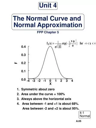
Standard normal curve properties • Why is it 'standard'? • Consider its equation: • What are three famous irrational numbers?
More properties of standard normal • Symmetric (about zero) • Monotonically decreasing on positives • Monotonically increasing on negatives • Area under the curve? • Calculate the integral
Standard normal: Area under the curve http://allpsych.com/researchmethods/distributions.html
Area under the curve: Integral - Use integral to calculate the area under the curve - For a contiguous area under the curve, use integration limits that correspond to the endpoints of the area
Area under the curve - Table of integrals usually have one endpoint as (negative infinity) - How do we use these tables to determine the area under the curve from a to b, where a is finite?
Area under the curve Think of the differences of two intervals: We know both integrals on the left-hand side:
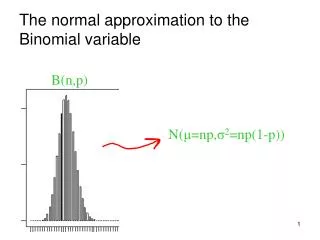
Normal approximation for data Assume that the population mean height (for men) is 69 inches • Population variance is 9 inches^2 • So, standard deviation is 3 inches • According to the normal approximation, what percentage of men have height between 66 inches and 72 inches?
Normal approximation • Mean height: 69 inches; SD = 3 inches • Translate 66 inches to 1 SD below the mean, since 69-3 = 66 • Translate 72 inches to 1 SD above the mean • Look back at the standard normal curve • See that about 68% of the area under the curve is within 1 sd of the mean
More on Normal approximation • How many SD's from the mean is an observed value? • Z value • For mean mu & SD sigma, and observed value x, • z is the number of standard deviations from the mean to the observation • Sign of z gives direction from mean to observation
Change of scale • What is the average of the numbers: 1,3,4,5,7 • What is their standard deviation? • For this calculation, use the equation: • Transform each original data point to a z-value: • What is the mean of the five z-values? • What is the standard deviation of the five z-values?
Lecture overview • Draw heavily on Freedman et al., Ch 5 • Normal curve • Areas under the normal curve • Normal approximation • Change of scale
Before Friday's lecture - Read carefully all of Chapter 5 in Freedman et al. - Review today's lecture materials - Freedman et al. has many exercises to practice these concepts. Do them. - Check your wisc.edu email - Homework 2 availability