~ Curve Fitting ~ Least Squares Regression Chapter 17
340 likes | 975 Vues
~ Curve Fitting ~ Least Squares Regression Chapter 17. Curve Fitting. Fit the best curve to a discrete data set and obtain estimates for other data points Two general approaches:

~ Curve Fitting ~ Least Squares Regression Chapter 17
E N D
Presentation Transcript
~ Curve Fitting ~Least Squares Regression Chapter 17
Curve Fitting • Fit the best curve to a discrete data set and obtain estimates for other data points • Two general approaches: • Data exhibit a significant degree of scatter Find a single curve that represents the general trend of the data. • Data is very precise. Pass a curve(s) exactly through each of the points. • Two common applications in engineering: Trend analysis. Predicting values of dependent variable: extrapolation beyond data points or interpolation between data points. Hypothesis testing. Comparing existing mathematical model with measured data.
Simple Statistics In sciences, if several measurements are made of a particular quantity, additional insight can be gained by summarizing the data in one or more well chosen statistics: Arithmetic mean - The sum of the individual data points (yi) divided by the number of points. Standard deviation – a common measure of spread for a sample or variance Coefficient of variation – quantifies the spread of data (similar to relative error)
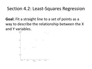
Linear Regression • Fitting a straight line to a set of paired observations: (x1, y1), (x2, y2),…,(xn, yn) yi: measured value e : error yi = a0 + a1 xi + e e = yi - a0 - a1 xi a1: slope a0: intercept e Error Line equation y = a0 + a1 x
Choosing Criteria For a “Best Fit” • Minimize the sum of the residual errors for all available data? Inadequate! (see ) • Sum of the absolute values? Inadequate! (see ) • How about minimizing the distance that an individual point falls from the line? This does not work either! see Regression line
e Error • Best strategy is to minimize the sum of the squares of the residuals between the measured-y and the y calculated with the linear model: • Yields a unique line for a given set of data • Need to compute a0 and a1 such that Sr is minimized!
Least-Squares Fit of a Straight Line Normal equations which can be solved simultaneously
Least-Squares Fit of a Straight Line Normal equations which can be solved simultaneously Mean values
“Goodness” of our fit • The spread of data • around the mean • around the best-fit line • Notice the improvement in the error due to linear regression • Sr = Sum of the squares of residuals around the regression line • St = total sum of the squares around the mean • (St – Sr) quantifies the improvement or error reduction due to describing data in terms of a straight line rather than as an average value. • For a perfect fitSr=0 and r = r2 = 1 signifies that the line explains 100 percent of the variability of the data. • For r = r2 = 0Sr=St the fit represents no improvement r : correlation coefficient r2 : coefficient of determination
Data that is ill-suited for linear least-squares regression • Indication that a parabola may be more suitable Exponential Eq. Linearization of Nonlinear Relationships
Saturation growth-rate Eq. Power Eq. Linearization of Nonlinear Relationships
Data to be fit to the power equation: Linear Regression yields the result: log y = 1.75*log x – 0.300 After (log y)–(log x) plot is obtained Find a2 and b2 using: b2 = 1.75 log a2 = - 0.3 a2 = 0.5 See Exercises.xls
Polynomial Regression • Some engineering data is poorly represented by a straight line. A curve (polynomial) may be better suited to fit the data. The least squares method can be extended to fit the data to higher order polynomials. • As an example let us consider a second order polynomial to fit the data points:
Polynomial Regression • To fit the data to an mth order polynomial, we need to solve the following system of linear equations ((m+1) equations with (m+1) unknowns) Matrix Form
Multiple Linear Regression • A useful extension of linear regression is the case where y is a linear function of two or more independent variables. For example: y = ao + a1x1 + a2x2 • For this 2-dimensional case, the regression line becomes a plane as shown in the figure below.
Multiple Linear Regression Which method would you use to solve this Linear System of Equations?
Multiple Linear Regression Example 17.6 The following data is calculated from the equation y = 5 + 4x1 - 3x2 Use multiple linear regression to fit this data. Solution: this system can be solved using Gauss Elimination. The result is: a0=5 a1=4 and a2= -3 y = 5 + 4x1 -3x2