Chapter 4 Interpolation and Approximation
Chapter 4 Interpolation and Approximation. 4.1 Lagrange Interpolation. The basic interpolation problem can be posed in one of two ways:. exist. unique. Example 4.1. e -1/2. Discussion . The construction presented in this section is called Lagrange interpolation .

Chapter 4 Interpolation and Approximation
E N D
Presentation Transcript
4.1 Lagrange Interpolation • The basic interpolation problem can be posed in one of two ways:
exist unique
Example 4.1 e-1/2
Discussion • The construction presented in this section is called Lagrange interpolation. • How good is interpolation at approximating a function? (Sections 4.3, 4.11) • Consider another example: • If we use a fourth-degree interpolating polynomial to approximate this function, the results are as shown in Figure 4.3 (a).
n= 8 n= 4 n= 16 Error for n=8
Discussion • There are circumstances in which polynomial interpolation as approximation will work very well, and other circumstances in which it will not. • The Lagrange form of the interpolating polynomial is not well suited for actual computations, and there is an alternative construction that is far superior to it.
4.2 Newton Interpolation and Divided Differences • The disadvantage of the Lagrange form • If we decide to add a point to the set of nodes, we have to completely re-compute all of the functions. • Here we introduce an alternative form of the polynomial: the Newton form • It can allow us to easily write in terms of
Discussion • The coefficients are called divided differences. • We can use divided-difference table to find them.
4.5 Application: More Approximations to the Derivative depends on x
4.5 Application: More Approximations to the Derivative • The interpolating polynomial in Lagrange form is • The error is given as in (4.20), thus • We get
4.7 Piecewise Polynomial Interpolation • If we keep the order of the polynomial fixed and use different polynomials over different intervals, with the length of the intervals getting smaller and smaller, then interpolation can be a very accurate and powerful approximation tool. • For example:
4.8 An Introduction to Splines • 4.8.1 Definition of the problem
Discussion • From the definition: • d: degree of approximation • Related to the number of unknown coefficients (the degrees of freedom) • N: degree of smoothness • Related to the number of constraints
Discussion • We can make the first term vanish by setting • This establishes a relationship between the polynomial degree of the spline and the smoothness degree. • For example: cubic splines • If we consider the common case of cubic splines, then d=3 and N=2.
4.8.2 Cubic B-Splines • B-Spline: assume an uniform grid
Cubic B-Splines • How do we know that B(x) is a cubic spline function? • Computer the one-sided derivatives at the knots: and similarly for the second derivative. • If the one-sided values are equal to each other, then the first and second derivatives are continuous, and hence B is a cubic spline. • Note that B is only “locally defined,” meaning that it is nonzero on only a small interval.
A Spline Approximation • We can use B to construct a spline approximation to an arbitrary function f. • Define the sequence of functions
xi=0.75 h=0.05 xi=0.4 h=0.05
A Spline Approximation • Now, we need to come up with two additional constraints in order to eliminate two of the unknowns. • Two common choices are • The natural spline: • A simple construction • Leads to higher error near the end points • The complete spline: • Better approximation properties • Do not actually require the derivative at the end points
From n-1 Natural Spline
From n+1 Complete Spline

