Lecture 5 Polynomial Approximation
Lecture 5 Polynomial Approximation. Polynomial Interpolation Example Limitation Polynomial Approximation (fitting) Line fitting Quadratic curve fitting Polynomial fitting. Polynomials. Polynomial determined by zeros in [-4,0,3]. P=poly([-4 0 3]);. Plot polynomial P. x=linspace(-5,5);

Lecture 5 Polynomial Approximation
E N D
Presentation Transcript
Lecture 5 Polynomial Approximation • Polynomial Interpolation • Example • Limitation • Polynomial Approximation (fitting) • Line fitting • Quadratic curve fitting • Polynomial fitting 數值方法
Polynomials Polynomial determined by zeros in [-4,0,3] P=poly([-4 0 3]); Plot polynomial P x=linspace(-5,5); y=polyval(P,x); plot(x,y); 數值方法
Sampling of paired data Produce a polynomial with zeros [-4,0,3] P=poly([-4 0 3]); Plot paired data x=rand(1,6)*10-5; y=polyval(P,x); plot(x,y, 'ro'); 數值方法
Polynomial interpolation Produce a polynomial with zeros [-4,0,3] P=poly([-4 0 3]); n=6 x=rand(1,n)*10-5; y=polyval(P,x); plot(x,y, 'ro'); Plot the interpolating polynomial v=linspace(min(x),max(x)); z=int_poly(v,x,y); plot(v,z,'k'); 數值方法
Demo_ip Source codes 數值方法
m=3, n=5 >> demo_ip data size n=5 數值方法
m=3, n=6 >> demo_ip data size n=6 數值方法
m=3, n=10 >> demo_ip data size n=10 數值方法
m=3, n=12 >> demo_ip data size n=12 數值方法
Sample with noise Produce a polynomial with zeros [-4,0,3] P=poly([-4 0 3]);n=6; x=rand(1,n)*10-5; y=polyval(P,x); nois=rand(1,n)*0.5-0.25; plot(x,y+nois, 'ro'); Plot the interpolating polynomial v=linspace(min(x),max(x)); z=int_poly(v,x,y+nois); plot(v,z,'k'); 數值方法
Demo_ip_noisy source codes 數值方法
Noise data • Noise ratio • Mean of abs(noise)/abs(signal) noise_ratio = 0.0074 數值方法
Numerical results Small noise causes intolerant interpolation >> demo_ip_noisy data size n:12 noise_ratio = 0.0053 數值方法
Numerical results Small noise causes intolerant interpolation >> demo_ip_noisy data size n:13 noise_ratio = 0.0031 數值方法
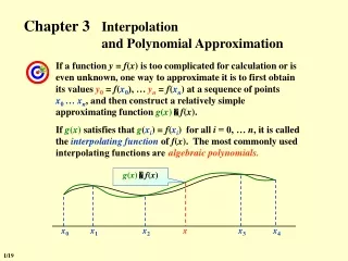
Interpolation Vs approximation • An interpolating polynomial is expected to satisfy all constraints posed by paired data • An interpolating polynomial is unable to retrieve an original target function when noisy paired data are provided • For noisy paired data, the goal of polynomial fitting is revised to minimize the mean square approximating error 數值方法
Polynomial approximation Given paired data, (xi,yi), i=1,…,n, the approximating polynomial is required to minimize the mean square error of approximating yi by f(xi) 數值方法
Polynomial fitting fa1d_polyfit.m 數值方法
Line fitting Minimizaing the mean square approximating error Target: 數值方法
Line fitting >> fa1d_polyfit input a function: x.^2+cos(x) :x+5 keyin sample size:300 polynomial degree:1 E = 8.3252e-004 Red: Approximating polynomial a=1;b=5 數值方法
Line fitting >> fa1d_polyfit input a function: x.^2+cos(x) :3*x+1/2 keyin sample size:30 polynomial degree:1 E = 0.0010 Red: Approximating polynomial a=3;b=1/2 數值方法
Objective function I • Line fitting Target: 數值方法
E1 is a quadratic function of a and b Setting derivatives of E1 to zero leads to a linear system 數值方法
a linear system 數值方法
Objective function II • Quadratic polynomial fitting Target: 數值方法
E2 are quadratic Setting derivatives of E2 to zero leads to a linear system 數值方法
a linear system 數值方法
Quadratic polynomial fitting • Minimization of an approximating error Target: 數值方法
Quadratic poly fitting input a function: x.^2+cos(x) :3*x.^2-2*x+1 keyin sample size:20 polynomial degree:2 E = 6.7774e-004 a=3 b=-2 c=1 數值方法
Data driven polynomial approximation • Minimization of Mean square error (mse) • Data driven polynomial approximation • f : a polynomial pm • Polynomial degree m is less than data size n 數值方法
POLYFIT: Fit polynomial to data • polyfit(x,y,m) • x : input vectors or predictors • y : desired outputs • m : degree of interpolating polynomial • Use m to prevent from over-fitting • Tolerance to noise 數值方法
POLYFIT: Fit polynomial to data A polynomial determined by zeros in [-4,0,3] P=poly([-4 0 3]); n=20;m=3; x=rand(1,20)*10-5; y=polyval(P,x); nois=rand(1,20)*0.5-0.25; plot(x,y+nois, 'ro'); Plot the interpolating polynomial v=linspace(min(x),max(x)); p=polyfit(x,y+nois,m);hold on; plot(v,polyval(p,v),'k'); 數值方法
Non-polynomial • sin fx=inline('sin(x)'); n=20;m=3 x=rand(1,n)*10-5; y=fx(x); nois=rand(1,n)*0.5-0.25; plot(x,y+nois, 'ro');hold on 數值方法
Under-fitting m=3 v=linspace(min(x),max(x)); p=polyfit(x,y+nois,m);hold on; plot(v,polyval(p,v),'k'); Under-fitting due to approximating non-polynomial by low-degree polynomials 數值方法
Intolerant mse >> mean((polyval(p,x)-(y+nois)).^2) ans = 0.0898 Under-fitting causes intolerant mean square error 數值方法
Under-fitting m=4; v=linspace(min(x),max(x)); p=polyfit(x,y+nois,m);hold on; plot(v,polyval(p,v), 'b'); M=4 數值方法
Fitting non-polynomial >> fa1d_polyfit input a function: x.^2+cos(x) :sin(x) keyin sample size:50 polynomial degree:5 E = 0.0365 數值方法
Fitting non-polynomial >> fa1d_polyfit input a function: x.^2+cos(x) :tanh(x+2)+sech(x) keyin sample size:30 polynomial degree:5 E = 0.0097 數值方法