Population A: 10,000
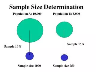
Sample Size Determination. Population A: 10,000. Population B: 5,000. Sample 15%. Sample 10%. Sample size 1000. Sample size 750. Sampling. The process of obtaining information from a subset (sample) of a larger group (population)

Population A: 10,000
E N D
Presentation Transcript
Sample Size Determination Population A: 10,000 Population B: 5,000 Sample 15% Sample 10% Sample size 1000 Sample size 750
Sampling • The process of obtaining information from a subset (sample) of a larger group (population) • The results for the sample are then used to make estimates of the larger group • Faster and cheaper than asking the entire population • Two keys • Selecting the right people • Have to be selected scientifically so that they are representative of the population • Selecting the right number of the right people • To minimize sampling errors I.e. choosing the wrong people by chance
Sample size Cost of research Selecting the right number of the right people • Three Issues • Financial • Managerial • Statistical Generally, the larger the sample size the smaller the statistical error, but the greater the cost, both financial and in terms of managerial resources
Male Female Totals <35 100 100 200 35+ 100 100 200 Totals 200 200 400 SubGroups The number of subgroups to be analyzed will have an impact on the size of the sample needed. As the number of subgroups increases the sampling error increases and it becomes harder to tell whether differences between two groups are real or due to error
Determining sample size Balance between financial and statistical issues 1. What can I afford 2. Rule of thumb past experience historical precedence gut feeling some consideration of sample error 3. Make up of sub-groups (cells) What statistical inferences do you hope to make between sub groups (rare to fall below 20 for a sub group) 4. Statistical Methods A critical factor will be the size of the expected difference or change to be measured, The smaller it is, the larger the sample needs to be.
Statistical determination • Three Pieces of Information Required • An estimate of the population Standard Deviation • The Acceptable Level of Sampling Error • The Desired Level of Confidence that the Sample Result will fall within a certain range (result +/- sampling error) of true population values
- a b Normal Distribution The height of a normal distribution can be uniquely specified mathematically in terms of two parameters: the mean (m) and the standard deviation (s).
IQ The total area under the curve is equal to 1. I.e. It takes in all observations The area of a region under the normal distribution between any two values equals the probability of observing a value in that range when an observation is randomly selected from the distribution For example, on a single draw there is a 34% chance of selecting from the distribution a person with an IQ between 100 and 115
Normal Distributions • Curve is basically bell shaped from - to • symmetric with scores concentrated in the middle (i.e. on the mean) than in the tails. • Mean, medium and mode coincide • They differ in how spread out they are.
Standard Normal Distribution (z) Any normal distribution can be converted into a standard normal distribution by a simple transformation formula. Z= value of the variable – Mean of variable/SD of the variable The mean always = zero; standard deviation always equal to one. The probabilities in the tables are always based on a normal distribution
Area Under Standard Normal Curve for Z values (Standard deviations) of 1, 2 and 3 Z values (Standard deviations) Area Under Standard Normal Curve % +/- 1 68.26 +/- 2 95.44 +/- 3 99.74
Population Vs. Sample Population of Interest Population Sample Parameter Statistic Sample We measure the sample using statistics in order to draw inferences about the population and its parameters. Population Mean = μ Standard Deviation Sample Mean = X Standard Deviation S
Sampling Distribution of the Mean • Necessary for understanding the basis for computing sampling error for simple random samples. • A conceptual and theoretical probability distribution of the means of all possible samples of a given size drawn from a given population • i.e. A distribution of sample means. • If you take a sample of 100 from a population of 1000 there are are thousands of different subsets of the population that can be drawn, each sample will have a slightly different mean. Those means will have also have a distribution. • Central Limit Theory says that that distribution will approximate a normal distribution the larger the number of samples drawn
Suppose you conducted a research study • Took a random sample of n=100 subjects • They tasted the new "Guacamole Doritos” • They rated the flavor of the chip on the following scale: • Too Perfect Too • Mild Flavor Hot 1 2 3 4 5 6 7
Results show : x1 = 2.3 and S1= 1.5 • Can you conclude that on average the target population thought the flavor was mild? • Suppose you take a series of random samples of n=100 subjects: • x2 = 3.7 and S2 = 2 • x3 = 4.3 and S3 = 0.5 • x4 = 2.8 and S4 = .97 • . • . • . • x50 = 3.7 and S50 = 2
X = (ΣXi)/n The Sampling Distribution The means of all the samples will have their own distribution called the sampling distribution of the means It is a normal distribution The mean of the sampling distribution of the mean = equals the population parameter
Sampling Distribution The standard deviation of the sampling distribution is called the sampling error of the mean Often the population standard deviation is unknown and has to be estimated from the sample S = Σ(Xi-X)/n-1 p= π(1-π)/n
Population distribution of the Doritos’ flavor (X) X Sample distribution of the x Doritos’ flavor x 1 2 3 4 5 6 7
What relationship does the Population Distribution have to the Sample Distribution? • The Central Limit Theorem • Let x1,x2….. xn denote a random sample selected from a population having mean and variance 2. Let X denote the sample mean. If n is large, the X has approximately a Normal Distribution with mean and variance 2/n. • The Central Limit Theorem does not mean that the sample mean = population mean. • It means that you can attach a probability to that value and decide.
X = / n • The sampling distribution of the mean for simple random samples that are over 30 has the following characteristics • The distribution is a normal distribution • The distribution has a mean equal to the population mean • The distribution has a standard deviation (the standard error of the mean ) equal to the population standard deviation divided by the square root of the sample size Note: The statistic is referred to as the standard error of the mean instead of the standard deviation to indicate that it applies to a distribution of sample means rather than the SD of a sample or of the population
Sampling Distribution of Proportions • We are often interested in estimating proportions or percentages rather than means • Is the sample proportion representative of the population proportion • The percentage of the population that has used the product • The percentage of the population that has purchased over the Internet in the last month • The proportion of men who read a particular magazine • The sampling distribution of the proportion approximates a normal distribution • The mean proportion of all possible samples is equal to the population proportion • The standard error of a sampling distribution cab be calculated
In practice we want to make inferences from our sample about the population it was drawn from • What is the probability that our sample of any given size will produce an estimate that is within one standard error (plus or minus) of the true population • The answer is 68.26% that any one sample from a particular population will produce an estimate of the population mean that is within +/- one standard error of the true value. • This is because 68.26% of all sample means from a given population fall in this range • There is a 95.44% probability that the mean from any one sample will within +/- two SDs
Sampling Distribution of Means Point Estimates • The sample mean is the best point estimate of a population mean • The sample mean is most likely to be close to the population mean, but could be any of the means on the left – including one that is a far distance from the population mean. • The distance between the sample mean and the population mean is the sampling error • Only a small percentage of samples will have the same mean as the population (I.e. a sampling error of zero)
Interval Estimates • Interval estimates are preferred • An interval estimate is a range of all values within which the true population mean is estimated to fall • Normally state the size of the interval, plus the probability that the interval will include the true population mean. • The probability is called the confidence level (e.g. 95%) • And the Interval is called the confidence interval (e.g. between 72 and 98)
Sample Confidence “Probability” we can take results as “accurate representation” of universe (i.e. that “sample statistics” are generalisable to the real “population parameters”) Typically a 95% probability (i.e. 19 times out of 20 we would expect results in this range)
Example: We can be 95% sure that, say, 65% of a target market will name Martini’s “V2” vodka in an unprompted recall test plus or minus 4%
We can be 95% sure (level ofconfidence) that, say, 65%(predicted result) of a target market (of a given total population) will name Martini’s “V2” vodka in an unprompted recall test plus or minus 4% (to a known margin of error)
95% confidence If we do the same test 20 times then it is statistically probable that the results will fall between 61-69 %, (i.e. 65 +/ 4%) at least 19 times If we lower the probability then we lower the sample error e.g.. at a 90% confidence level, result might be between 64% - 66% (a tighter range but we are less sure the sample is representative of the real population)
Implications for sample size (Given reliability and validity hold) Above a certain size little extra information is gathered by increasing the sample size. Generally, there is no relationship between the size of a population and the size of sample needed to estimate a particular population parameter, with a particular error range and level of confidence.
To determine Sample Size we need three pieces of information • The acceptable level of sampling error • The acceptable level of confidence • The estimate of the population standard deviation
Sample Size Determination • 3 Statistical Determinants of Sample Size • DEGREE OF CONFIDENCE • Statistical Confidence • 95% Confidence or .05 Level of Significance • DEGREE OF PRECISION • Accuracy in Estimating Population Proportion • +/- $5.00 versus +/- $1.00 • +/- 10% versus +/- 5% • VARIABILITY IN THE POPULATION • To What Degree do the Sampling Units Differ
We can choose an error range (e.g. + 5%) • We can set a confidence level (e.g. 95%) • But • Without knowing the spread of results (i.e. the standard deviation for the population) we cannot work out the sample size required • So • How can we estimate the population standard deviation before selecting the sample: • pilot tests • guess • previous experience • Secondary data n = Z2σ2 E2 Z = level of confidence σ = population SD E = acceptable amount of sampling error
Example • Number of fast food restaurant visits in past month • We need our estimate to be within 1/10 (.01) of a visit from the population average (E) • We need to be 95.44% confident that the true population mean falls in the interval defined by the sample mean plus or minus E (i.e. within 2 standard deviations) Z=2 • Standard deviation – guess at 1.39 days = 7.72 .01 n = Z2σ2 E2 = 22(1.39) 2 (01) 2 = 4(2.93) 2 .01 = 772
Sample Size Determination To be More confident More precise If more variable Sample size must increase Too big - it’s a waste of money Too small - you cannot make a big decision
Significance level In hypothesis testing, the significance level is the criterion used for rejecting the null hypothesis. The significance level is used as follows: First, the difference between the results of the experiment and the null hypothesis is determined. Then, assuming the null hypothesis is true, the probability of a difference that large or larger is computed. Finally, this probability is compared to the significance level. If the probability is less than or equal to the significance level, then the null hypothesis is rejected and the outcome is said to be statistically significant.
Traditionally, experimenters have used either the .05 level (sometimes called the 5% level) or the .01 level (1% level), although the choice of levels is largely subjective. The lower the significance level, the more the data must diverge from the null hypothesis to be significant. Therefore, the .01 level is more conservative than the .05 level. The Greek letter alpha is sometimes used to indicate the significance level.
/2 /2 -2.023 2.816 0 2.023 Critical value • A critical value is the value that a test statistic must exceed in order for the the null hypothesis to be rejected. • For example, the critical value of t (with 12 degrees of freedom using the .05 significance level) is 2.18. • This means that for the probability value to be less than or equal to .05, the absolute value of the t statistic must be 2.18 or greater. critical value Significance level (.05) Test statistic
The t distribution • The t distribution is used instead of the normal distribution whenever the standard deviation is estimated. • The t distribution has relatively more scores in its tails than does the normal distribution. • The shape of the t distribution depends on the degrees of freedom (df) that went into the estimate of the standard deviation. • As the degrees of freedom increases, the t distribution approaches the normal distribution. • With 100 or more degrees of freedom, the t distribution is almost indistinguishable from the normal distribution.