Runoff generation and its representation in land surface models
900 likes | 1.08k Vues
Dennis P. Lettenmaier Department of Civil and Environmental Engineering University of Washington for presentation at GSSP Seminar Series NASA/GSFC June 14, 2002. Runoff generation and its representation in land surface models. 1. Runoff generation processes

Runoff generation and its representation in land surface models
E N D
Presentation Transcript
Dennis P. Lettenmaier Department of Civil and Environmental Engineering University of Washington for presentation at GSSP Seminar Series NASA/GSFC June 14, 2002 Runoff generation and its representation in land surface models
1. Runoff generation processes 2. Spatially distributed modeling 3. Macroscale modeling a) Strategy b) Testing and evaluation c) Implementation Example 1 – Puget Sound flood forecast system Example 2 – Seasonal ensemble forecasting Example 3 – Climate change assessment OUTLINE OF THIS TALK
Darcy’s Equation (fundamental equation of motion in subsurface, applies to both saturated and unsaturated zones): whereq = flow per unit cross-sectional area (units L/T) K = hydraulic conductivity (L/T) Definitions: = volume of water/total volume η = porosity (volume of voids/total volume = suction head (height to which moisture is drawn above free surface
let = diffusivity From continuity Combining, (Richard’s equation)
Applies at point scale, “well behaved” porous medium K is highly nonlinear spatially varying function of suction head, moisture K varies over orders of magnitude due to variations in soil properties at meter scales (much less than typical scale of application) Direct estimation of K difficult even at small scale (and scale complications in interpretation of measurements) Methods of estimating K from e.g. mapable soil properties are highly approximate, and subject to scale complications Complications in the application of Richards Equation
1) Infiltration excess – precipitation rate exceeds local (vertical) hydraulic conductivity -- typically occurs over low permeability surfaces, e.g., arid areas with soil crusting, frozen soils 2) Saturation excess – “fast” runoff response over saturated areas, which are dynamic during storms and seasonally (defined by interception of the water table with the surface) Runoff generation mechanisms
Runoff generation mechanisms on a hillslope (source: Dunne and Leopold)
Seasonal contraction of saturated area at Sleepers River, VT following snowmelt (source: Dunne and Leopold)
Expansion of saturated area during a storm (source: Dunne and Leopold)
Seasonal contraction of pre-storm saturated areas, Sleepers River VT (source: Dunne and Leopold)
2. Spatially distributed modeling Distributed Hydrology Soil Vegetation Model (DHSVM)
Explicit Representation of Downslope Moisture Redistribution Lumped Conceptual (Processes parameterized)
Smaller Sub-watersheds More realistic Processes • Streamflow (at predetermined points) • Predictive skill limited to calibration conditions Streamflow Snow Runoff Soil Moisture, etc at all points and areas in the basin Predictive Skill Outside Calibration Conditions. Distributed vs Spatially Lumped Hyrologic Models Lumped Conceptual Fully Distributed Physically-based Suitable for flood forecasting and a wide range of water resource related issues Suitable for flood forecasting
Traditional “bottom up” hydrologic modeling approach (subbasin by subbasin)
Macroscale modeling approach (“top down”) 1 Northwest 5 Rio Grande 10 Upper Mississippi 2 California 6 Missouri 11 Lower Mississippi 3 Great Basin 7 Arkansas-Red 12 Ohio 4 Colorado 8 Gulf 13 East Coast 9 Great Lakes
3. Macroscale hydrologic models, • b: Testing and evaluation
Investigation of forest canopy effects on snow accumulation and melt Measurement of Canopy Processes via two 25 m2 weighing lysimeters (shown here) and additional lysimeters in an adjacent clear-cut. Direct measurement of snow interception
Calibration of an energy balance model of canopy effects on snow accumulation and melt to the weighing lysimeter data. (Model was tested against two additional years of data)
Summer 1994 - Mean Diurnal Cycle Rnet Rnet 300 Rnet 100 -100 250 H H 150 H 50 -50 120 LE LE LE 60 0 0 3 6 9 12 15 18 21 24 0 3 6 9 12 15 18 21 24 0 3 6 9 12 15 18 21 24 Observed Fluxes Simulated Fluxes Rnet Net Radiation H Sensible Heat Flux LE Latent Heat Flux Point Evaluation of a Surface Hydrology Model for BOREAS SSA Mature Black Spruce NSA Mature Black Spruce SSA Mature Jack Pine Flux (W/m2) Local time (hours)
Eurasia North America ) 20 10 2 km 6 16 8 12 6 snow cover extent (10 8 4 4 2 0 0 J F M A M J J A S O N D J J F M A M J J A S O N D J Month Month Observed Simulated Range in Snow Cover Extent Observed and Simulated
UPPER LAYER SOIL MOISTURE Illinois soil moisture comparison 0.40 TOPLATS regional ESTAR distributed X TOPLATS distributed 0.30 X SOIL MOISTURE (%) X X X X 0.20 X X X X X X X X X X 0.10 June 18th-July 20th, 1997 11:00 CST JUNE 20, 1997 11:00 CST JULY 12 1997 50 50 10 10 ESTAR TOPLATS ESTAR TOPLATS
A B C D 200 Soil Moisture (mm) Normalized 100 0 J F M A M J J A S O N D J J F M A M J J A S O N D J J F M A M J J A S O N D J J F M A M J J A S O N D J E F G H 200 Soil Moisture (mm) Normalized 100 0 J F M A M J J A S O N D J J F M A M J J A S O N D J J F M A M J J A S O N D J J F M A M J J A S O N D J Observed Simulated 60°N 60°N E H A D G 50°N 50°N B C F 40°N 40°N 20°E 30°E 40°E 50°E 60°E 70°E 80°E 90°E 100°E 110°E 120°E 130°E 140°E Mean Normalized Observed and Simulated Soil Moisture Central Eurasia, 1980-1985
Cold Season Parameterization -- Frozen Soils Key Observed Simulated 5-100 cm layer 0-5 cm layer
Terrain - 150 m. aggregated from 10 m. resolution DEM • Land Cover - 19 classes aggregated from over 200 GAP classes • Soils - 3 layers aggregated from 13 layers (31 different classes); variable soil depth from 1-3 meters • Stream Network - based on 0.25 km2 source area Data Requirements for applying DHSVM.
Calibration-Validation with all available meteorological observations (50 sites) Validation 1991-1996 Calibration (Snohomish River) From 1987-1991 (USGS gauges at Gold Bar and Carnation only )
Principal calibration locations were the Skykomish at Gold Bar and the Snoqualmie at Carnation DHSVM Calibration (Snoqualmie at Carnation) Flood of record
Calibration Location (Snoqualmie) Testing: Cedar • Calibration to two USGS sites • Split sample validation at over 60 sites • Parameters transfer extremely well to other watersheds without recalibration
2000/2001 Real-time Streamflow Forecast System 26 basins 48,896 km2 2,173,155 pixels @ 150 m resolution http://hydromet.atmos.washington.edu
The average relative absolute error in peak runoff forecast for six events during water year 1999 (Westrick et al 2002). Obs-based MM5 MM5 no bias RFC Sauk Skykomish N.F. Snoq M.F. Snoq Snoq Cedar