Download
1 / 1
10 likes | 213 Vues
Enhanced Oil Recovery using Coupled Electromagnetics and Flow Modelling . E. Haber, UBC (haber@math.ubc.ca) E. Holtham Computational Geosciences Inc (elliot@compgeoinc.com). INTRODUCTION

E N D
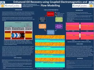
Enhanced Oil Recovery using Coupled Electromagnetics and Flow Modelling E. Haber, UBC (haber@math.ubc.ca) E. Holtham Computational Geosciences Inc (elliot@compgeoinc.com) INTRODUCTION Enhanced Oil Recovery (EOR) is a process in which gas or fluid is injected into a reservoir in order to push oil into a production well. A sketch of this process is shown below. There are several aspects for such a process. One of the most important issues is the ability to control the flow and direct it into the direction that would lead to the recovery of crude oil. In principle, the flow of water/gas/oil can be modeled using variety of techniques and therefore, the flow can be predicted. However, in practice, the flow equations contain parameters that are unknown and therefore, prediction is difficult and in many cases, highly inaccurate. FLOW and ELECTROMAGNETICS • EM MODELLING • Layered conductive model with a thin resistive reservoir. • Grounded electrodes, one end down the bore-hole and the other end grounded 2km away • Transmitter position moved in 7.5 m increments along the bore-hole • Current injection below the reservoir, inside the reservoir, and above the reservoir. • Synthetic data at four different time steps of the injection process were modeled. • Data inverted in 3D porosity hydraulic conductivity capillary pressure mobility functions initial conditions1 500 m 1 km Initial 5 days Enhanced Oil Recovery: Water and CO2 are flooded through an injection well. The CO2 mobilizes additional oil that can be recovered at a production well. Figure from the Kansas Geological Survey. 10 days 15 days Inverted conductivity models at different time steps CONCLUSIONS Simulations of a flooding event were modeled using geologic and hydraulic parameters of an oil field. The flow simulations demonstrate the capability to accurately predict the movement of CO2 in the reservoir given a good estimate of the hydrological parameters of a reservoir. To enhance the EM inversion results, the outputs of the flow simulation software were used as constraints for the electromagnetic inversions. Once the constraint model was constructed, the data were inverted in 3D. The changes in the inverted conductivity models image the injection event over time. Given a sufficient conductivity difference between the different CO2 injection time steps, along with an appropriate survey geometry, the modeling results demonstrate that EM methods are feasible for monitoring oil recovery processes. To alleviate this problem and to better control the flow, imaging can be used. In particular, remote time lapse monitoring of reservoirs can provide valuable information to meet production goals. Remote monitoring requires technology that can detect movement and changes in the reservoir during production and flooding events. Flooding events can be modeled and monitored. Here we present a methodology combining flow simulation software and electromagnetic data that can yield accurate control of the flow. First the injection event is simulated to predict the fluid flow. This information is then used as a constraint when inverting the collected geophysical data. The combination of flow simulation and electromagnetic data inversion provides an enhanced monitoring technique for reservoir characterization. • FLOW Modelling • Modeling the flow can be done by using the pressure-saturation equations. This is a highly coupled systems of PDE's. Here, we consider the formulation suggested by Friis and S. Evje (2012). • Discretize the equations in space first using a cell-centered controlled volume • Integrate in time using Implicit Pressure Explicit Saturation (IMPES) algorithm • First solve the pressure equation to compute velocity • Integrate the hyperbolic equation for the saturation using an implicit upwind method • Yields an effective flow simulator that can be used for electromagnetic inversion REFERENCES R. Amestoy, I.S. Du, J.-Y. L'Excellent, and J. Koster. A fully asynchronous multifrontalsolver using distributed dynamic scheduling. simax, 23:15-41,2001. H.A. Friis and S. Evje. Numerical treatment of two-phase flow in capillary heterogeneous porous media by finite volume approximations. Int. J. Num. Anal. Mod, 9:505-36, 2012. E. Haber and S. Heldmann. An octreemultigrid method for quasi-static Maxwell's equations with highly discontinuous coefficients. Journal of Computational Physics, 65:324-337, 2007. E. Haber, D. Oldenburg, and R. Shektman. Inversion of time domain 3D electromagnetic data. Geophysical Journal International, 132:1324-1335, 2007. G. R. Hjaltason and H. Samet. Speeding up construction of Quadtrees for spatial indexing. The VLDB Journal, 11:109- 137, 2002. L. Horesh and E. Haber. A second order discretization of Maxwell's equations in the quasi-static regime on Octreegrids. SIAM J. Sci. Comput, 33:2805 A2822, 2011. C. Schwarzbach and E. Haber. Finite element based inversion for time-harmonic electromagnetic problems. submitted, 2011. K.S. Yee. Numerical solution of initial boundary value problems involving Maxwell's equations in isotropic media. IEEE Trans. on antennas and propagation, 14:302-307, 1966. Time lapse images of the injection using the flow simulation software