Characterization of Forecast Error using Singular Value Decomposition
Characterization of Forecast Error using Singular Value Decomposition. Andy Moore and Kevin Smith University of California Santa Cruz Hernan Arango Rutgers University. Outline. An overview of singular value decomposition (SVD) Flavors of SVD Duality of SVD Norms Unstable jet

Characterization of Forecast Error using Singular Value Decomposition
E N D
Presentation Transcript
Characterization of Forecast Error using Singular Value Decomposition Andy Moore and Kevin Smith University of California Santa Cruz Hernan Arango Rutgers University
Outline • An overview of singular value decomposition (SVD) • Flavors of SVD • Duality of SVD • Norms • Unstable jet • California Current
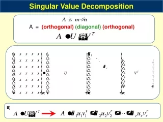
Singular Value Decomposition (SVD) A generalization of eigenvectors for rectangular matrices. Square Matrix: Rectangular Matrix: Right singular vectors: Left singular vectors: Important rank/ dimension info
v2 v1 Think Covariance! A u2 u1
SVD and “Model” Errors State vector: Perfect model: Imperfect model: Error Errors: TLM: Tangent linear model
Singular Value Decomposition (SVD) Complimentary Function (CF) Particular integral (PI) SVD of CF – Singular vectors of initial conditions (i.e. ECMWF EFS) Final Time Covariance at t=t Initial Condition Covariance at t=0 SV 2 SV 2 SV 1 SV 1
Singular Value Decomposition (SVD) Complimentary Function (CF) Particular integral (PI) SVD of PI – Stochastic optimals (SO) Model Error Covariance at t=t Model Error Covariance at t~0 SO 2 (q2) SO 2 (q2) SO 1 (q1) SO 1 (q1)
Duality of SVD Fastest growing perturbations Fastest growing errors Dynamics of meander and eddy formation Most predictable patterns Fastest loss of predictability
Flavors of SVD Initial condition error: Find the e0 that maximizes: FInal time norm Subject to the constraint: Initial time norm Equivalent to the generalized eigenvalue problem: and SVD of:
Illustrative Example – A Zonal Jet 500m deep, f=10-4, b=0, Dx-15km, Dz=100m Eastward Gaussian jet, 40km width, 1.6ms-1 SV time interval = 2 days. Energy norm, P=C. 600km Initial SV 360km SVD: Forcing SV SVD: Stoch Opt (white) SVD: Stoch Opt (red) SVD: tc= 2 days
Conservation of wave action (or pseudomomentum): Doppler shifting of (w-ku) is accompanied by increase in E (Buizza and Palmer, 1995). Periodic Channel & Zonal Jet y y x x z z x x Initial Final
Baroclinically Unstable Jet t=0 t=50 days 2000km SST SST Dx=10km, f=-10-4, b=1.6×10⁻¹¹ 1000km SH
Initial Condition Singular Vectors Singular Vector #12 Singular Vector #12 t=0 t=2 days SSH SSH Singular Vector #11 Singular Vector #11 t=0 t=2 days SSH SSH Energy norm at initial and final time
? The Forecast Problem Forecast Error Covariance at t=t Analysis Error Covariance at t=0 SV 2 SV 2 forecast F Ea SV 1 SV 1 t=T t=0 Perform SVD on: Forecast initial condition error= analysis error subject to: (Ehrendorfer & Tribbia, 1998)
The Inverse Analysis Error Covariance, (Ea)-1 Prior Error Cov. Adjoint of ROMS Obs Error Cov. Tangent of ROMS Inverse Analysis error covariance Hessian matrix Primal space Lanczos vector expansion from 4D-Var Hessian matrix The number Lanczos vectors = number of 4D-Var inner-loops
The Forecast Error Covariance, F Experience in numerical weather prediction at ECMWF suggests that F=E is a good choice (Buizza and Palmer, 1995). We will assume the same here… … more on this later however…
Evolved Analysis Error Covariance (Ea)-1 (Ea)-1 t0 ta tf Ma Mf Analysis cycle (4D-Var) Forecast cycle
Evolved Analysis Error Covariance We actually need the analysis error at the end of the analysis cycle: so we need the time evolved Lanczos vectors, Ve. but Reorthonormalize using Gramm-Schmidt: where: and
The dimension of the problem is reduced to the # of 4D-Var inner- loops whole spectrum. Hessian Singular Vectors Find the x that maximizes forecast error Subject to the constraint that (Barkmeijer et al, 1998) But Solve the equivalent eigenvalue problem: where (Cholesky factorization of T) and and where A+ is the right generalized inverse, and
Baroclinically Unstable Jet: Identical Twin 4D-Var Strong constraint primal 4D-Var 1 outer-loop, 15 inner-loops 2 day assimilation window Perfect T obs everywhere on day 0, day 1, day 2 Initial conditions only adjusted Balance operator applied
No assim No assim No assim No assim 4D-Var 4D-Var 4D-Var 4D-Var Forecast Forecast Forecast Forecast rms error in SSH rms error in T Cycle # Cycle # rms error in u rms error in v Cycle # Cycle #
SVn SVn SV1 SV1 SVn SVn SV1 SV1 Singular Values of 2 Day Jet Forecasts SV # log10l Cycle #
SVn SVn Rugby Ball SV1 SV1 SVn SVn Cigar SV1 SV1
Hessian Singular Vectors SV #1 SV #1 Final SSH Final SSH Initial SSH Initial SSH CYCLE #1 CYCLE #20 SV #1 Final SSH Initial SSH CYCLE #40
Hessian Singular Vectors SV #1 CYCLE #1 Forecast SSH Final SSH Initial SSH t=2 days SV #1 CYCLE #20
The California Current ERA40 and CCMP forcing SODA open boundary conditions fb(t), Bf bb(t), Bb xb(0), Bx Previous assimilation cycle 30km, 10 km, 3 km & 1km grids, 30- 42 levels Veneziani et al (2009) Broquet et al (2009)
Observations (y) CalCOFI & GLOBEC SST & SSH Ingleby and Huddleston (2007) TOPP Elephant Seals Argo Data from Dan Costa
Sequential 4D-Var Observations Observations Observations prior prior prior 4D-Var Analysis 4D-Var Analysis 4D-Var Analysis Posterior Posterior Posterior 8 day 4D-Var cycles overlapping every 4 days
30 Year Reanalysis of California Current 1980-2010 Obs:Pathfinder, AMSR-E, MODIS, EN3, Aviso Forcing: ERA40, ERA-Interim, CCMP (25 km) Analysis every 4 days, 8 day overlapping assim cycles http://www.oceanmodeling.ucsc.edu Initial cost J Moore et al. (2012) Final cost J + Final NL J
SVn SVn Spring SV1 SV1 SVn SVn Autumn SV1 SV1 CCS: Hessian SVs 10 km CCS ROMS SV # log10l Jan 1999 June 1999 Dec 1999 Cycle #
SVn SVn Spring SV1 SV1 SVn SVn Autumn SV1 SV1
CYCLE #1 SV SSH initial Forecast SSH SV SSH final 10 km CCS ROMS
CYCLE #23 SV SSH initial Forecast SSH SV SSH final 10 km CCS ROMS
The Forecast Error Covariance Recall that we can express the forecast error cov. as: Forecast error covariance Tangent linear model Control priors where: Posterior error covariance Tangent Linear 4D-Var Adjoint Linear 4D-Var So the control SVD problem becomes: (computational cost equals (# inner-loops)2)
Summary • SVD provides information about • forecast error growth. • Growing directions of the forecast error • covariance error ellipsoid vary with time • SV structures become smaller scale • Flow and/or error dependent regimes • Future work: • - explicit forecast error covariance • - model error and weak constraint • - control singular vectors