Singular Value Decomposition
Singular Value Decomposition. Singular Value Decomposition. Homogeneous least-squares Span and null-space Closest rank r approximation Pseudo inverse. Singular Value Decomposition. Homogeneous least-squares. Parameter estimation. 2D homography
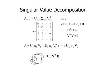

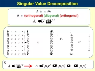
Singular Value Decomposition
E N D
Presentation Transcript
Singular Value Decomposition • Homogeneous least-squares • Span and null-space • Closest rank r approximation • Pseudo inverse
Singular Value Decomposition Homogeneous least-squares
Parameter estimation • 2D homography Given a set of (xi,xi’), compute H (xi’=Hxi) • 3D to 2D camera projection Given a set of (Xi,xi), compute P (xi=PXi) • Fundamental matrix Given a set of (xi,xi’), compute F (xi’TFxi=0) • Trifocal tensor Given a set of (xi,xi’,xi”), compute T
Number of measurements required • At least as many independent equations as degrees of freedom required • Example: 2 independent equations / point 8 degrees of freedom 4x2≥8
Approximate solutions • Minimal solution 4 points yield an exact solution for H • More points • No exact solution, because measurements are inexact (“noise”) • Search for “best” according to some cost function • Algebraic or geometric/statistical cost
Gold Standard algorithm • Cost function that is optimal for some assumptions • Computational algorithm that minimizes it is called “Gold Standard” algorithm • Other algorithms can then be compared to it
Direct Linear Transformation(DLT) • Equations are linear in h • Only 2 out of 3 are linearly independent (indeed, 2 eq/pt)
(only drop third row if wi’≠0) • Holds for any homogeneous representation, • e.g. (xi’,yi’,1)
Direct Linear Transformation(DLT) • Solving for H size A is 8x9 or 12x9, but rank 8 Trivial solution is h=09T is not interesting 1-D null-space yields solution of interest pick for example the one with
Direct Linear Transformation(DLT) • Over-determined solution No exact solution because of inexact measurement i.e. “noise” • Find approximate solution • Additional constraint needed to avoid 0, e.g. • not possible, so minimize
DLT algorithm • Objective • Given n≥4 2D to 2D point correspondences {xi↔xi’}, determine the 2D homography matrix H such that xi’=Hxi • Algorithm • For each correspondence xi ↔xi’ compute Ai. Usually only two first rows needed. • Assemble n 2x9 matrices Ai into a single 2nx9 matrix A • Obtain SVD of A. Solution for h is last column of V • Determine H from h
Inhomogeneous solution Since h can only be computed up to scale, pick hj=1, e.g. h9=1, and solve for 8-vector Solve using Gaussian elimination (4 points) or using linear least-squares (more than 4 points) However, if h9=0 this approach fails also poor results if h9 close to zero Therefore, not recommended Note h9=H33=0 if origin is mapped to infinity
Define: Then, Degenerate configurations x1 x1 x1 x4 x4 x4 x2 H? H’? x2 x2 x3 x3 x3 (case B) (case A) i=1,2,3,4 Constraints: H* is rank-1 matrix and thus not a homography If H* is unique solution, then no homography mapping xi→xi’(case B) If further solution H exist, then also αH*+βH (case A) (2-D null-space in stead of 1-D null-space)
3D Homographies (15 dof) Minimum of 5 points or 5 planes 2D affinities (6 dof) Minimum of 3 points or lines Solutions from lines, etc. 2D homographies from 2D lines Minimum of 4 lines Conic provides 5 constraints Mixed configurations?
Cost functions • Algebraic distance • Geometric distance • Reprojection error • Comparison • Geometric interpretation • Sampson error
algebraic distance where Algebraic distance DLT minimizes residual vector partial vector for each (xi↔xi’) algebraic error vector Not geometrically/statistically meaningfull, but given good normalization it works fine and is very fast (use for initialization)
measured coordinates estimated coordinates true coordinates Error in one image Symmetric transfer error Geometric distance d(.,.) Euclidean distance (in image) e.g. calibration pattern Reprojection error
typical, but not , except for affinities Comparison of geometric and algebraic distances Error in one image For affinities DLT can minimize geometric distance Possibility for iterative algorithm
Analog to conic fitting Geometric interpretation of reprojection error Estimating homography~fit surface to points X=(x,y,x’,y’)T in 4 represents 2 quadrics in 4 (quadratic in X)
Sampson error: 1st order approximation of Vector that minimizes the geometric error is the closest point on the variety to the measurement Find the vector that minimizes subject to Sampson error between algebraic and geometric error
Use Lagrange multipliers: minimize derivatives Find the vector that minimizes subject to
Sampson error: 1st order approximation of Vector that minimizes the geometric error is the closest point on the variety to the measurement Find the vector that minimizes subject to Sampson error between algebraic and geometric error (Sampson error)
Sampson approximation A few points • For a 2D homography X=(x,y,x’,y’) • is the algebraic error vector • is a 2x4 matrix, e.g. • Similar to algebraic error in fact, same as Mahalanobis distance • Sampson error independent of linear reparametrization (cancels out in between e and J) • Must be summed for all points • Close to geometric error, but much fewer unknowns
Maximum Likelihood Estimate Statistical cost function and Maximum Likelihood Estimation • Optimal cost function related to noise model • Assume zero-mean isotropic Gaussian noise (assume outliers removed) Error in one image
Maximum Likelihood Estimate Statistical cost function and Maximum Likelihood Estimation • Optimal cost function related to noise model • Assume zero-mean isotropic Gaussian noise (assume outliers removed) Error in both images
Error in two images (independent) Varying covariances Mahalanobis distance • General Gaussian case Measurement X with covariance matrix Σ
Invariance to transforms ? will result change? for which algorithms? for which transformations?
Non-invariance of DLT Given and H computed by DLT, and Does the DLT algorithm applied to yield ?
for similarities Effect of change of coordinates on algebraic error so
Non-invariance of DLT Given and H computed by DLT, and Does the DLT algorithm applied to yield ?
Invariance of geometric error Given and H, and Assume T’ is a similarity transformations
Or Normalizing transformations • Since DLT is not invariant, what is a good choice of coordinates? e.g. • Translate centroid to origin • Scale to a average distance to the origin • Independently on both images
Importance of normalization 1 ~104 ~102 ~102 ~102 ~102 ~102 1 ~104 orders of magnitude difference!
Normalized DLT algorithm • Objective • Given n≥4 2D to 2D point correspondences {xi↔xi’}, determine the 2D homography matrix H such that xi’=Hxi • Algorithm • Normalize points • Apply DLT algorithm to • Denormalize solution
Iterative minimization metods Required to minimize geometric error • Often slower than DLT • Require initialization • No guaranteed convergence, local minima • Stopping criterion required Therefore, careful implementation required: • Cost function • Parameterization (minimal or not) • Cost function ( parameters ) • Initialization • Iterations
Parameterization Parameters should cover complete space and allow efficient estimation of cost • Minimal or over-parameterized? e.g. 8 or 9 (minimal often more complex, also cost surface) (good algorithms can deal with over-parameterization) (sometimes also local parameterization) • Parametrization can also be used to restrict transformation to particular class, e.g. affine
Function specifications • Measurement vector XNwith covariance Σ • Set of parameters represented by vector P N • Mapping f: M →N. Range of mapping is surface S representing allowable measurements • Cost function: squared Mahalanobis distance Goal is to achieve , or get as close as possible in terms of Mahalanobis distance
Symmetric transfer error Error in one image Reprojection error
Initialization • Typically, use linear solution • If outliers, use robust algorithm • Alternative, sample parameter space
Iteration methods Many algorithms exist • Newton’s method • Levenberg-Marquardt • Powell’s method • Simplex method
Gold Standard algorithm • Objective • Given n≥4 2D to 2D point correspondences {xi↔xi’}, determine the Maximum Likelyhood Estimation of H • (this also implies computing optimal xi’=Hxi) • Algorithm • Initialization: compute an initial estimate using normalized DLT or RANSAC • Geometric minimization of -Either Sampson error: • ● Minimize the Sampson error • ● Minimize using Levenberg-Marquardt over 9 entries of h • or Gold Standard error: • ● compute initial estimate for optimal {xi} • ● minimize cost over {H,x1,x2,…,xn} • ● if many points, use sparse method
Robust estimation • What if set of matches contains gross outliers?
RANSAC • Objective • Robust fit of model to data set S which contains outliers • Algorithm • Randomly select a sample of s data points from S and instantiate the model from this subset. • Determine the set of data points Si which are within a distance threshold t of the model. The set Si is the consensus set of samples and defines the inliers of S. • If the subset of Si is greater than some threshold T, re-estimate the model using all the points in Si and terminate • If the size of Si is less than T, select a new subset and repeat the above. • After N trials the largest consensus set Si is selected, and the model is re-estimated using all the points in the subset Si
Distance threshold Choose t so probability for inlier is α (e.g. 0.95) • Often empirically • Zero-mean Gaussian noise σ then follows distribution with m=codimension of model (dimension+codimension=dimension space)
How many samples? Choose N so that, with probability p, at least one random sample is free from outliers. e.g. p=0.99
Acceptable consensus set? • Typically, terminate when inlier ratio reaches expected ratio of inliers
Adaptively determining the number of samples e is often unknown a priori, so pick worst case, e.g. 50%, and adapt if more inliers are found, e.g. 80% would yield e=0.2 • N=∞, sample_count =0 • While N >sample_count repeat • Choose a sample and count the number of inliers • Set e=1-(number of inliers)/(total number of points) • Recompute N from e • Increment the sample_count by 1 • Terminate