Download
1 / 54
540 likes | 766 Vues
7. Economic Growth I: Capital Accumulation and Population Growth. In this chapter, you will learn…. the closed economy Solow model how a country’s standard of living depends on its saving and population growth rates

E N D
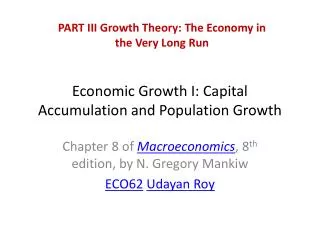
7 Economic Growth I: Capital Accumulation and Population Growth
In this chapter, you will learn… • the closed economy Solow model • how a country’s standard of living depends on its saving and population growth rates • how to use the “Golden Rule” to find the optimal saving rate and capital stock CHAPTER 7 Economic Growth I
Why growth matters • Data on infant mortality rates: • 20% in the poorest 1/5 of all countries • 0.4% in the richest 1/5 • In Pakistan, 85% of people live on less than $2/day. • One-fourth of the poorest countries have had famines during the past 3 decades. • Poverty is associated with oppression of women and minorities. Economic growth raises living standards and reduces poverty…. CHAPTER 7 Economic Growth I
annual growth rate of income per capita percentage increase in standard of living after… Why growth matters • Anything that effects the long-run rate of economic growth – even by a tiny amount – will have huge effects on living standards in the long run. …25 years …100 years …50 years 169.2% 2.0% 64.0% 624.5% 2.5% 85.4% 243.7% 1,081.4% CHAPTER 7 Economic Growth I
Why growth matters • If the annual growth rate of U.S. real GDP per capita had been just one-tenth of one percent higher during the 1990s, the U.S. would have generated an additional $496 billion of income during that decade. CHAPTER 7 Economic Growth I
The lessons of growth theory …can make a positive difference in the lives of hundreds of millions of people. These lessons help us • understand why poor countries are poor • design policies that can help them grow • learn how our own growth rate is affected by shocks and our government’s policies CHAPTER 7 Economic Growth I
The Solow model • due to Robert Solow,won Nobel Prize for contributions to the study of economic growth • a major paradigm: • widely used in policy making • benchmark against which most recent growth theories are compared • looks at the determinants of economic growth and the standard of living in the long run CHAPTER 7 Economic Growth I
How Solow model is different from Chapter 3’s model 1.K is no longer fixed:investment causes it to grow, depreciation causes it to shrink 2.L is no longer fixed:population growth causes it to grow 3. the consumption function is simpler CHAPTER 7 Economic Growth I
How Solow model is different from Chapter 3’s model 4.no G or T(only to simplify presentation; we can still do fiscal policy experiments) 5.cosmetic differences CHAPTER 7 Economic Growth I
The production function • In aggregate terms: Y = F (K, L) • Define: y = Y/L = output per worker k = K/L = capital per worker • Assume constant returns to scale:zY = F (zK, zL ) for any z > 0 • Pick z = 1/L. Then Y/L = F (K/L, 1) y = F (k, 1) y = f(k) where f(k) = F(k, 1) CHAPTER 7 Economic Growth I
Output per worker, y f(k) MPK = f(k +1) – f(k) 1 Capital per worker, k The production function Note: this production function exhibits diminishing MPK. CHAPTER 7 Economic Growth I
The national income identity • Y = C + I (remember, no G ) • In “per worker” terms: y = c + iwhere c = C/L and i = I/L CHAPTER 7 Economic Growth I
The consumption function • s = the saving rate, the fraction of income that is saved (s is an exogenous parameter) Note: s is the only lowercase variable that is not equal to its uppercase version divided by L • Consumption function: c = (1–s)y(per worker) CHAPTER 7 Economic Growth I
Saving and investment • saving (per worker) = y – c = y – (1–s)y = sy • National income identity is y = c + i Rearrange to get: i = y – c = sy(investment = saving, like in chap. 3!) • Using the results above, i = sy = sf(k) CHAPTER 7 Economic Growth I
Output per worker, y f(k) c1 sf(k) y1 i1 Capital per worker, k k1 Output, consumption, and investment CHAPTER 7 Economic Growth I
Depreciation per worker, k k 1 Capital per worker, k Depreciation = the rate of depreciation = the fraction of the capital stock that wears out each period CHAPTER 7 Economic Growth I
Capital accumulation The basic idea: Investment increases the capital stock, depreciation reduces it. Change in capital stock = investment – depreciation k = i– k Since i = sf(k) , this becomes: k = sf(k)– k CHAPTER 7 Economic Growth I
The equation of motion for k k = sf(k)– k • The Solow model’s central equation • Determines behavior of capital over time… • …which, in turn, determines behavior of all of the other endogenous variables because they all depend on k. E.g., income per person: y = f(k) consumption per person: c = (1–s)f(k) CHAPTER 7 Economic Growth I
The steady state k = sf(k)– k If investment is just enough to cover depreciation [sf(k)=k ], then capital per worker will remain constant: k = 0. This occurs at one value of k, denoted k*, called the steady state capital stock. CHAPTER 7 Economic Growth I
Investment and depreciation k sf(k) k* Capital per worker, k The steady state CHAPTER 7 Economic Growth I
Investment and depreciation k sf(k) k investment depreciation k1 k* Capital per worker, k Moving toward the steady state k = sf(k) k CHAPTER 7 Economic Growth I
Investment and depreciation k sf(k) k k* k1 Capital per worker, k Moving toward the steady state k = sf(k) k k2 CHAPTER 7 Economic Growth I
Investment and depreciation k sf(k) k investment depreciation k* Capital per worker, k Moving toward the steady state k = sf(k) k k2 CHAPTER 7 Economic Growth I
Investment and depreciation k sf(k) k k* Capital per worker, k Moving toward the steady state k = sf(k) k k2 k3 CHAPTER 7 Economic Growth I
Investment and depreciation k sf(k) k* Capital per worker, k Moving toward the steady state k = sf(k) k Summary:As long as k < k*, investment will exceed depreciation, and k will continue to grow toward k*. k3 CHAPTER 7 Economic Growth I
Now you try: Draw the Solow model diagram, labeling the steady state k*. On the horizontal axis, pick a value greater than k* for the economy’s initial capital stock. Label it k1. Show what happens to k over time. Does k move toward the steady state or away from it? CHAPTER 7 Economic Growth I
A numerical example Production function (aggregate): To derive the per-worker production function, divide through by L: Then substitute y = Y/L and k = K/L to get CHAPTER 7 Economic Growth I
A numerical example, cont. Assume: • s = 0.3 • = 0.1 • initial value of k = 4.0 CHAPTER 7 Economic Growth I
Approaching the steady state: A numerical example Year k y c i k k 1 4.000 2.000 1.400 0.600 0.400 0.200 2 4.200 2.049 1.435 0.615 0.420 0.195 3 4.395 2.096 1.467 0.629 0.440 0.189 4 4.584 2.141 1.499 0.642 0.458 0.184 … 10 5.602 2.367 1.657 0.710 0.560 0.150 … 25 7.351 2.706 1.894 0.812 0.732 0.080 … 100 8.962 2.994 2.096 0.898 0.896 0.002 … 9.000 3.000 2.100 0.900 0.900 0.000 CHAPTER 7 Economic Growth I
Exercise: Solve for the steady state Continue to assume s = 0.3, = 0.1, and y = k 1/2 Use the equation of motion k = s f(k) kto solve for the steady-state values of k, y, and c. CHAPTER 7 Economic Growth I
Solution to exercise: CHAPTER 7 Economic Growth I
Investment and depreciation k s2 f(k) s1 f(k) k An increase in the saving rate An increase in the saving rate raises investment… …causing k to grow toward a new steady state: CHAPTER 7 Economic Growth I
Prediction: • Higher s higher k*. • And since y = f(k) , higher k* higher y* . • Thus, the Solow model predicts that countries with higher rates of saving and investment will have higher levels of capital and income per worker in the long run. CHAPTER 7 Economic Growth I
International evidence on investment rates and income per person 100,000 Income per person in 2000 (log scale) 10,000 1,000 100 0 5 10 15 20 25 30 35 Investment as percentage of output (average 1960-2000) CHAPTER 7 Economic Growth I
The Golden Rule: Introduction • Different values of s lead to different steady states. How do we know which is the “best” steady state? • The “best” steady state has the highest possible consumption per person: c* = (1–s) f(k*). • An increase in s • leads to higher k* and y*, which raises c* • reduces consumption’s share of income (1–s), which lowers c*. • So, how do we find the s and k* that maximize c*? CHAPTER 7 Economic Growth I
The Golden Rule capital stock the Golden Rule level of capital, the steady state value of kthat maximizes consumption. To find it, first express c* in terms of k*: c* = y*i* = f(k*)i* = f(k*)k* In the steady state: i*=k* because k = 0. CHAPTER 7 Economic Growth I
steady state output and depreciation k* f(k*) steady-state capital per worker, k* The Golden Rule capital stock Then, graph f(k*) and k*, look for the point where the gap between them is biggest. CHAPTER 7 Economic Growth I
k* f(k*) The Golden Rule capital stock c*= f(k*) k*is biggest where the slope of the production function equals the slope of the depreciation line: MPK = steady-state capital per worker, k* CHAPTER 7 Economic Growth I
The transition to the Golden Rule steady state • The economy does NOT have a tendency to move toward the Golden Rule steady state. • Achieving the Golden Rule requires that policymakers adjust s. • This adjustment leads to a new steady state with higher consumption. • But what happens to consumption during the transition to the Golden Rule? CHAPTER 7 Economic Growth I
time Starting with too much capital then increasing c* requires a fall in s. In the transition to the Golden Rule, consumption is higher at all points in time. y c i t0 CHAPTER 7 Economic Growth I
Starting with too little capital then increasing c* requires an increase in s. Future generations enjoy higher consumption, but the current one experiences an initial drop in consumption. y c i t0 time CHAPTER 7 Economic Growth I
Population growth • Assume that the population (and labor force) grow at rate n. (n is exogenous.) • EX: Suppose L = 1,000 in year 1 and the population is growing at 2% per year (n = 0.02). • Then L = nL = 0.021,000 = 20,so L = 1,020 in year 2. CHAPTER 7 Economic Growth I
Break-even investment • ( +n)k = break-even investment, the amount of investment necessary to keep k constant. • Break-even investment includes: • k to replace capital as it wears out • nk to equip new workers with capital (Otherwise, k would fall as the existing capital stock would be spread more thinly over a larger population of workers.) CHAPTER 7 Economic Growth I
actual investment break-even investment The equation of motion for k • With population growth, the equation of motion for k is k = sf(k) (+n)k CHAPTER 7 Economic Growth I
Investment, break-even investment (+n)k sf(k) k* Capital per worker, k The Solow model diagram k=s f(k) ( +n)k CHAPTER 7 Economic Growth I
(+n2)k sf(k) k2* The impact of population growth Investment, break-even investment (+n1)k An increase in n causes an increase in break-even investment, leading to a lower steady-state level of k. k1* Capital per worker, k CHAPTER 7 Economic Growth I
Prediction: • Higher n lower k*. • And since y = f(k) , lower k* lower y*. • Thus, the Solow model predicts that countries with higher population growth rates will have lower levels of capital and income per worker in the long run. CHAPTER 7 Economic Growth I
International evidence on population growth and income per person Income 100,000 per Person in 2000 (log scale) 10,000 1,000 100 0 1 2 3 4 5 Population Growth (percent per year; average 1960-2000) CHAPTER 7 Economic Growth I
The Golden Rule with population growth To find the Golden Rule capital stock, express c* in terms of k*: c* = y*i* = f(k* ) ( + n)k* c* is maximized when MPK = + n or equivalently, MPK = n In the Golden Rule steady state, the marginal product of capital net of depreciation equals the population growth rate. CHAPTER 7 Economic Growth I