Model Checking I I
Model Checking I I. How CTL model checking works. CTL. A E X F G U Model checking problem Determine M, s0 f Or find all s s.t. M, s f. Need only the boolean connectives ( , ) and

Model Checking I I
E N D
Presentation Transcript
Model Checking II How CTL model checking works
CTL A E X F G U Model checking problem Determine M, s0 f Or find alls s.t. M, s f
Need only the boolean connectives ( , ) and E X F G U define others e.g. AG p EF p A(p U q) E( q U p & q) & EG( q) (Could skip EF and define in terms of EU, but hopefully seeing how EF is done aids understanding)
Explicit state model checking Option 1 CES (original paper) Represent state transition graph explicitly Walk around marking states Graph algorithms involving strongly connected components etc. Not covered in this course (cf. SPIN) Used particularly in software model checking
Symbolic MC Option 2 McMillan et al because of STATE EXPLOSION problem State graph exponential in program/circuit size Graph algorithms linear in state graph size INSTEAD Use symbolic representation of both sets of states and of state transtion graph
Symbolic MC Sets of states formulas relations between states (BDDs) Fixed point characerisations of CTL ops NO explicit state graph
A state Vector of boolean variables (v1,v2,v3, …., vn) {0,1}n
Boolean formulas (x y) z ( is exclusive or) (1 0) 0 = 1 assignment [x=1,y=0,z=0] gives answer 1 is a model or satisfying assignment Write as 100 Exercise: Find another model
Boolean formulas (x y) z (1 1) 0 = 0 assignment [x=1,y=1,z=0] is not a model
Formula is a tautology if ALL assignments are models and is contradictory if NONE is.
Boolean formulas For us, interesting formulas are somewhere in between: some assignments are models, some not IDEA: A formula can represent a set of states (its models)
{} false {111} x y z {101} x y z {111,101} x z . . {000,001, … , 111} true
Example (x y) z represents {100,010,001,111} for states of the form xyz Exercise: Find formulas (with var. names x,y,z) for the sets {} {100} {110,100,010,000}
What is needed now? A good data structure for boolean formulas Binary Decision Diagrams (BDDs) Lee (Bell Systems Tech. Journal 59) Akers (IEEE Trans. Comp 78) Bryant (IEEE Trans. Comp. 86, most cited CS paper!) see also Bryant’s document about a Hitachi patent from 93 McMillan saw application to symbolic MC
Binary Decision Diagrams Canonical form (constant time comparison) Polynomial algorithms for ’and’, ’or’, ’not’ etc. Exponential but practically efficient algorithm for boolean quantification (even of sets of variables) Read Hu’s excellent tutorial paper (See Course Literature) (Presentation based on lecture notes by Ken McMillan)
Ordered Decision Tree ab + cd (ab) (cd) a 0 1 b b 0 1 0 1 c c c c 0 1 0 1 0 1 0 1 d d d d d d d d 0 0 0 1 0 0 0 1 0 0 0 1 1 1 1 1
To get OBDD Combine isomorphic subtrees Eliminate redundant nodes (those with identical children) Tree becomes a graph
(O)BDD ab + cd (ab) (cd) a 1 0 b 0 c 1 d 0 0 1 0 1
Make BDD for (x y) z
Combinational equivalence checking For two circuits with single boolean outputs, make BDDs for each circuit and see if they are the same Of course the BDDs are built up by application of BDD construction functions and, or, not etc. NOT by making decision tree and then reducing
BDDs + Many formulas (and circuits) have small representations -Some do not! Multipliers - BDD representation of a function can vary exponentially in size depending on variable ordering; users may need to play with variable orderings (less automatic) + Good algorithms and packages (e.g. CUDD) + EXTREMELY useful in practice - Size limitations a big problem
Represent a set of states Just make the BDD for a corresponding formula!
Represent a transition relation R Remember that R is just a set of pairs of states Use two sets of variables, v and v’ (with the primed variables representing next states) Make a formula involving both v and v’ and from that a BDD bdd(R,(v,v’))
What set of states can we reach from set P in one step? R R R R P Image(P,R) {t s s P s R t}
Forward Image R R R R P Image(P,R) {t s s P s R t} bdd(Image(P,R),v’) = v bdd(P,v) bdd(R,(v,v’))
Backward image R R R R Q {s t t Q s R t} bdd(Image-1(Q,R),v) = v’ bdd(Q,v’) bdd(R,(v,v’))
So far BDDs for • sets of states • transition relation • calculating forward or backward image of a set Need one last idea: iteration to a fixed point based on recursive description of CTL ops
Symbolic MC of CTL Compute set of states satisfying a formula recursively (and use BDDs as rep.) consider , , EX, EF, EG, EU define others
CTL formula f H(f) set of states satisfying f a (atomic) L(a) (cf.Lars) p S – H(p) p qH(p) H(q) EX p familiar ?
CTL formula f H(f) set of states satisfying f EX p Image-1(H(p),R)
CTL formula f bdd for set of states satisfying f EX p v’bdd(p,v’) bdd(R,(v,v’))
Remaining operators Recursive characterisation EF p p EX (EF p)
CTL EF p p EX (EF p) Start with the empty set of states, , as a first guess, and improve it by applying p EX (.) to it
Fixed point iteration (formulas) S0 = false S1 = pEX (false)=p S2 = pEX (p) S3 = pEX (pEX (p)) and so on Will eventually terminate. Why?
Now think sets S0 = Ø = empty set of states S1 = H(p)Image-1(Ø,R) =H(p) S2 = H(p)Image-1(H(p),R) Si+1 = H(p) Image-1(Si,R) Will eventually terminate. Why?
Fixed point iteration p EX p P
Fixed point iteration p EX (p EX p) P
Fixed point iteration Evetually stops! P . . . .
LEAST fixed point Started with a small set (empty, indeed) and made it larger. All ok because F(B) = H(p) Image-1(B,R) is monotonic (i.e. if B B’ then F(B) F(B’)) Write least y s.t. y = F(y) as y.F(y)
EG EG p p EX (EG p) This time need to work downwards
Fixed point iteration (formulas) S0 = true S1 = pEX (true) S2 = pEX (pEX (true)) and so on Will eventually terminate. Why?
Now think sets S0 = S = the entire set of states S1 = H(p) Image-1(S,R) S2 = H(p) Image-1(H(p) Image-1(S,R) ,R) Si+1 = H(p) Image-1(Si,R) Will eventually terminate.
Greatest fixed point EG p p EX (EG p) H(EG p) = y. H(p) Image-1(y,R)
EG EG p p EX (EG p) H(EG p) = y. H(p) Image-1(y,R) NB: We can do all of these operations using BDDs to represent the sets
Fixed point interationin the other direction p EX (p EX p) P
Fixed point interationin the other direction p EX (p EX p) …. p
EU E (p U q) q (p EX (E (p U q)) H(E (p U q)) = y. H(q) (H(p) Image-1(y,R)) This is a generalisation of the EF case. Remember that E (True U q) = EF q Exercise: define H (A(p U q)). See earlier slide

