Maps, Hash Tables and Dictionaries
500 likes | 722 Vues
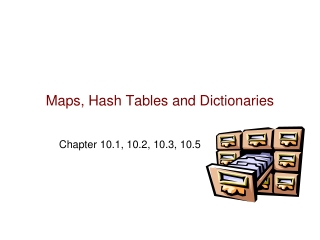
Maps, Hash Tables and Dictionaries. Chapter 10.1, 10.2, 10.3, 10.5. Outline. Maps Hashing Dictionaries Ordered Maps & Dictionaries. Outline. Maps Hashing Dictionaries Ordered Maps & Dictionaries. Maps. A map models a searchable collection of key-value entries

Maps, Hash Tables and Dictionaries
E N D
Presentation Transcript
Maps, Hash Tables and Dictionaries Chapter 10.1, 10.2, 10.3, 10.5
Outline Maps Hashing Dictionaries Ordered Maps & Dictionaries
Outline Maps Hashing Dictionaries Ordered Maps & Dictionaries
Maps • A map models a searchable collection of key-value entries • The main operations of a map are for searching, inserting, and deleting items • Multiple entries with the same key are not allowed • Applications: • address book • student-record database
The Map ADT • Map ADT methods: • get(k): if the map M has an entry with key k, return its associated value; else, return null • put(k, v): insert entry (k, v) into the map M; if key k is not already in M, then return null; else, return old value associated with k • remove(k): if the map M has an entry with key k, remove it from M and return its associated value; else, return null • size(), isEmpty() • keys(): return an iterator over the keys in M • values(): return an iterator of the values in M • entries(): returns an iterator over the entries in M
Example Operation Output M isEmpty() true Ø put(5,A) null (5,A) put(7,B) null (5,A),(7,B) put(2,C) null (5,A),(7,B),(2,C) put(8,D) null (5,A),(7,B),(2,C),(8,D) put(2,E) C (5,A),(7,B),(2,E),(8,D) get(7) B (5,A),(7,B),(2,E),(8,D) get(4) null (5,A),(7,B),(2,E),(8,D) get(2) E (5,A),(7,B),(2,E),(8,D) size() 4 (5,A),(7,B),(2,E),(8,D) remove(5) A (7,B),(2,E),(8,D) remove(2) E (7,B),(8,D) get(2) null (7,B),(8,D) isEmpty() false (7,B),(8,D)
Comparison with java.util.Map Map ADT Methodsjava.util.Map Methods size() size() isEmpty() isEmpty() get(k) get(k) put(k,v) put(k,v) remove(k) remove(k) keys() keySet() values() values() entries()entrySet()
We could implement a map using an unsorted list We store the entries of the map in a doubly-linked list S, in arbitrary order S supports the node list ADT (Section 6.2) A Simple List-Based Map trailer nodes/positions header a d 5 8 c b 9 6 entries
The get(k) Algorithm Algorithm get(k): B =S.positions() {B is an iterator of the positions in S} while B.hasNext() do p=B.next()// the next position in B if p.element().getKey() = k then return p.element().getValue() return null {there is no entry with key equal to k}
The put(k,v) Algorithm Algorithm put(k,v): B =S.positions() while B.hasNext() do p=B.next() if p.element().getKey() = k then t =p.element().getValue() S.set(p,(k,v)) return t{return the old value} S.addLast((k,v)) n=n+ 1 {increment variable storing number of entries} return null {there was no previous entry with key equal to k}
The remove(k) Algorithm Algorithm remove(k): B =S.positions() while B.hasNext() do p=B.next() if p.element().getKey() = k then t =p.element().getValue() S.remove(p) n = n – 1 {decrement number of entries} return t{return the removed value} return null {there is no entry with key equal to k}
Performance: put, getand remove take O(n) time since in the worst case (the item is not found) we traverse the entire sequence to look for an item with the given key The unsorted list implementation is effective only for small maps Performance of a List-Based Map
Outline Maps Hashing Dictionaries Ordered Maps & Dictionaries
Hash Tables A hash table is a data structure that can be used to make map operations faster. While worst-case is still O(n), average case is typically O(1).
Applications of Hash Tables databases compilers browser caches
A hash functionh maps keys of a given type to integers in a fixed interval [0, N- 1] Example:h(x) =x mod Nis a hash function for integer keys The integer h(x) is called the hash value of key x A hash table for a given key type consists of Hash function h Array (called table) of size N When implementing a map with a hash table, the goal is to store item (k, o) at index i=h(k) Hash Functions and Hash Tables
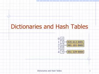
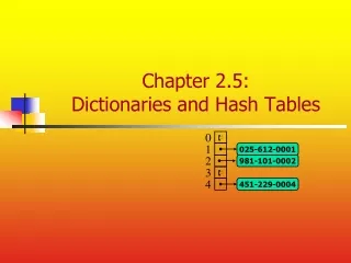
Example • We design a hash table for a map storing entries as (SIN, Name), where SIN (social insurance number) is a nine-digit positive integer • Our hash table uses an array of sizeN= 10,000 and the hash functionh(x) = last four digits of SIN x 0 Ø 1 025-612-0001 2 981-101-0002 3 Ø 4 451-229-0004 … 9997 Ø 9998 200-751-9998 9999 Ø
Hash Functions A hash function is usually specified as the composition of two functions: Hash code:h1:keysintegers Compression function:h2: integers[0, N- 1] The hash code is applied first, and the compression function is applied next on the result, i.e., h(x) = h2(h1(x)) The goal of the hash function is to “disperse” the keys in an apparently random way
Hash Codes • Memory address: • We reinterpret the memory address of the key object as an integer (default hash code of all Java objects) • Does not work well when copies of the same object may be stored at different locations. • Integer cast: • We reinterpret the bits of the key as an integer • Suitable for keys of length less than or equal to the number of bits of the integer type (e.g., byte, short, int and float in Java) • Component sum: • We partition the bits of the key into components of fixed length (e.g., 16 or 32 bits) and we sum the components (ignoring overflows) • Suitable for keys of fixed length greater than or equal to the number of bits of the integer type (e.g., long and double in Java)
Problems with Component Sum Hash Codes • Hashing works when • the number of different common keys is small relative to the hashing space (e.g., 232 for a 32-bit hash code). • the hash codes for common keys are well-distributed (do not collide) in this space. • Component Sum codes ignore the ordering of the components. • e.g., using 8-bit ASCII components, ‘stop’ and ‘pots’ yields the same code. • Since common keys are often anagrams of each other, this is often a bad idea!
Polynomial Hash Codes • Polynomial accumulation: • We partition the bits of the key into a sequence of components of fixed length (e.g., 8, 16 or 32 bits)a0 a1 … an-1 • We evaluate the polynomial p(z)= a0+a1 z+a2 z2+ …+an-1zn-1 at a fixed value z, ignoring overflows • Especially suitable for strings • Polynomial p(z) can be evaluated in O(n) time using Horner’s rule: • The following polynomials are successively computed, each from the previous one in O(1) time p0(z)= an-1 pi(z)= an-i-1 +zpi-1(z) (i=1, 2, …, n-1) • We have p(z) = pn-1(z)
Compression Functions • Division: • h2 (y) =ymod N • The size N of the hash table is usually chosen to be a prime (on the assumption that the differences between hash keys y are less likely to be multiples of primes). • Multiply, Add and Divide (MAD): • h2 (y) = [(ay + b)mod p] mod N, where • p is a prime number greater than N • a and b are integers chosen at random from the interval [0, p – 1], with a > 0.
Collision Handling 0 Ø 1 025-612-0001 2 Ø 3 Ø 4 451-229-0004 981-101-0004 • Collisions occur when different elements are mapped to the same cell • Separate Chaining: • Let each cell in the table point to a linked list of entries that map there • Separate chaining is simple, but requires additional memory outside the table
Map Methods with Separate Chaining • Delegate operations to a list-based map at each cell: Algorithmget(k): Output: The value associated with the key kin the map, or null if there is no entry with key equal to kin the map return A[h(k)].get(k) {delegate the get to the list-based map at A[h(k)]}
Map Methods with Separate Chaining • Delegate operations to a list-based map at each cell: Algorithmput(k,v): Output:Store the new (key, value) pair. If there is an existing entry with key equal to k, return the old value; otherwise, return null t=A[h(k)].put(k,v) {delegate the put to the list-based map at A[h(k)]} if t= null then {kis a new key} n=n+ 1 return t
Map Methods with Separate Chaining • Delegate operations to a list-based map at each cell: Algorithmremove(k): Output: The (removed) value associated with key kin the map, or null if there is no entry with key equal to kin the map t=A[h(k)].remove(k) {delegate the remove to the list-based map at A[h(k)]} if t≠null then {kwas found} n=n - 1 return t
Open addressing: the colliding item is placed in a different cell of the table Linear probinghandles collisions by placing the colliding item in the next (circularly) available table cell Each table cell inspected is referred to as a “probe” Colliding items lump together, so that future collisions cause a longer sequence of probes Example: h(x) =xmod13 Insert keys 18, 41, 22, 44, 59, 32, 31, 73, in this order Open Addressing: Linear Probing 41 18 44 59 32 22 31 73 0 1 2 3 4 5 6 7 8 9 10 11 12
Consider a hash table A of length Nthat uses linear probing get(k) We start at cell h(k) We probe consecutive locations until one of the following occurs An item with key k is found, or An empty cell is found, or N cells have been unsuccessfully probed Get with Linear Probing Algorithmget(k) ih(k) p0 repeat cA[i] if c=Ø returnnull else if c.key() =k returnc.element() else i(i+1)mod N pp+1 untilp=N returnnull
Suppose we receive a remove(44) message. What problem arises if we simply remove the key = 44 entry? Example: h(x) =xmod13 Insert keys 18, 41, 22, 44, 59, 32, 31, 73, in this order Remove with Linear Probing Ø ✗ 41 18 44 59 32 22 31 73 0 1 2 3 4 5 6 7 8 9 10 11 12
Removal with Linear Probing Algorithmget(k) ih(k) p0 repeat cA[i] if c=Ø returnnull else if c.key() =k returnc.element() else i(i+1)mod N pp+1 untilp=N returnnull To address this problem, we introduce a special object, calledAVAILABLE , which replaces deleted elements AVAILABLE has a null key No changes to get(k) are required.
Updates with Linear Probing • remove(k) • We search for an entry with key k • If such an entry (k, o) is found, we replace it with the special item AVAILABLE and we return element o • Else, we return null • put(k, o) • We throw an exception if the table is full • We start at cell h(k) • We probe consecutive cells until one of the following occurs • A cell i is found that is either empty or stores AVAILABLE, or • N cells have been unsuccessfully probed • We store entry (k, o) in cell i
Open Addressing: Double Hashing • Double hashing is an alternative open addressing method that uses a secondary hash function h’(k)in addition to the primary hash function h(x). • Suppose that the primary hashing i=h(k) leads to a collision. • We then iteratively probe the locations(i+ jh’(k)) mod N for j= 0, 1, … , N - 1 • The secondary hash functionh’(k) cannot have zero values • N is typically chosen to be prime. • Common choice of secondary hash function h’(k): • h’(k) = q- k mod q, where • q< N • q is a prime • The possible values for h’(k) are1, 2, … , q
Example of Double Hashing • Consider a hash table storing integer keys that handles collision with double hashing • N= 13 • h(k) =kmod13 • h’(k) =7 -kmod7 • Insert keys 18, 41, 22, 44, 59, 32, 31, 73 31 41 18 32 59 73 22 44 0 1 2 3 4 5 6 7 8 9 10 11 12
Example of Double Hashing • Consider a hash table storing integer keys that handles collision with double hashing • N= 13 • h(k) =kmod13 • h’(k) =7 -kmod7 • Insert keys 18, 41, 22, 44, 59, 32, 31, 73 31 41 18 32 59 73 22 44 0 1 2 3 4 5 6 7 8 9 10 11 12
Performance of Hashing • In the worst case, searches, insertions and removals on a hash table take O(n) time • The worst case occurs when all the keys inserted into the map collide • The load factorλ=n/N affects the performance of a hash table • For separate chaining, performance is typically good for λ < 0.9. • For open addressing , performance is typically good for λ < 0.5. • java.util.HashMap maintains λ < 0.75 • Open addressing can be more memory efficient than separate chaining, as we do not require a separate data structure. • However, separate chaining is typically as fast or faster than open addressing.
Rehashing • When the load factor λ exceeds threshold, the table must be rehashed. • A larger table is allocated (typically at least double the size). • A new hash function is defined. • All existing entries are copied to this new table using the new hash function.
Outline Maps Hashing Dictionaries
The dictionary ADT models a searchable collection of key-element entries The main operations of a dictionary are searching, inserting, and deleting items Multiple items with the same key are allowed Applications: word-definition pairs credit card authorizations Dictionary ADT methods: get(k): if the dictionary has at least one entry with key k, returns one of them, else, returns null getAll(k): returns an iterable collection of all entries with key k put(k, v): inserts and returns the entry (k, v) remove(e): removes and returns the entry e. Throws an exception if the entry is not in the dictionary. entrySet(): returns an iterable collection of the entries in the dictionary size(), isEmpty() Dictionary ADT
Dictionaries and Java Note: The java.util.Dictionary class actually implements a map ADT. There is no dictionary data structure in the Java Collections Framework that supports multiple entries with equal keys. The textbook (Section 9.5.3) provides an implementation of a Dictionary based upon a map of keys, each entry of which supports a linked list of entries with the same key.
Example Operation Output Dictionary put(5,A) (5,A) (5,A) put(7,B) (7,B) (5,A),(7,B) put(2,C) (2,C) (5,A),(7,B),(2,C) put(8,D) (8,D) (5,A),(7,B),(2,C),(8,D) put(2,E) (2,E) (5,A),(7,B),(2,C),(8,D),(2,E) get(7) (7,B) (5,A),(7,B),(2,C),(8,D),(2,E) get(4) null (5,A),(7,B),(2,C),(8,D),(2,E) get(2) (2,C) (5,A),(7,B),(2,C),(8,D),(2,E) getAll(2) (2,C),(2,E)(5,A),(7,B),(2,C),(8,D),(2,E) size() 5 (5,A),(7,B),(2,C),(8,D),(2,E) remove(get(5)) (5,A) (7,B),(2,C),(8,D),(2,E) get(5) null (7,B),(2,C),(8,D),(2,E)
Subtleties of remove(e) Operation Output Dictionary e1 = put(2,C) (2,C) (5,A),(7,B),(2,C) e2 = put(8,D) (8,D) (5,A),(7,B),(2,C),(8,D) e3 = put(2,E) (2,E) (5,A),(7,B),(2,C),(8,D),(2,E) remove(get(5)) (5,A) (7,B),(2,C),(8,D),(2,E) remove(e3)(2,E) (7,B),(2,C),(8,D) remove(e1)(2,C) (7,B),(8,D) remove(e) will remove an entry that matches e (i.e., has the same (key, value) pair). If the dictionary contains more than one entry with identical (key, value) pairs, remove(e) will only remove one. Example:
A log file or audit trail is a dictionary implemented by means of an unsorted sequence We store the items of the dictionary in a sequence (based on a doubly-linked list or array), in arbitrary order Performance: insert takes O(1) time since we can insert the new item at the beginning or at the end of the sequence find and remove take O(n) time since in the worst case (the item is not found) we traverse the entire sequence to look for an item with the given key The log file is effective only for dictionaries of small size or for dictionaries on which insertions are the most common operations, while searches and removals are rarely performed (e.g., historical record of logins to a workstation) A List-Based Dictionary
The getAll and put Algorithms Algorithm put(k,v) Create a new entry e = (k,v) S.addLast(e) {S is unordered} return e Algorithm getAll(k) Create an initially-empty list L for e: D do if e.getKey() = k then L.addLast(e) return L
The remove Algorithm Algorithm remove(e): { We don’t assume here that e stores its position in S } B = S.positions() while B.hasNext() do p = B.next() if p.element() = e then S.remove(p) return e return null {there is no entry e in D}
Hash Table Implementation • We can also create a hash-table dictionary implementation. • If we use separate chaining to handle collisions, then each operation can be delegated to a list-based dictionary stored at each hash table cell.
Outline Maps Hashing Dictionaries Ordered Maps & Dictionaries
Ordered Maps and Dictionaries • If keys obey a total order relation, can represent a map or dictionary as an ordered search table stored in an array. • Can then support a fast find(k) using binary search. • at each step, the number of candidate items is halved • terminates after a logarithmic number of steps • Example: find(7) 0 1 3 4 5 7 8 9 11 14 16 18 19 m h l 0 1 3 4 5 7 8 9 11 14 16 18 19 m h l 0 1 3 4 5 7 8 9 11 14 16 18 19 m h l 0 1 3 4 5 7 8 9 11 14 16 18 19 l=m =h
Performance: find takes O(logn) time, using binary search insert takes O(n) time since in the worst case we have to shift nitems to make room for the new item remove takes O(n) time since in the worst case we have to shift nitems to compact the items after the removal A search table is effective only for dictionaries of small size or for dictionaries on which searches are the most common operations, while insertions and removals are rarely performed (e.g., credit card authorizations) Ordered Search Tables
Summary: Learning Outcomes • Maps • ADT • What are they good for? • Naïve implementation – running times • Hashing • Running time • Types of hashing • Dictionaries • ADT • What are they good for? • Ordered Maps & Dictionaries • What are they good for? • Running time