Hash Tables
Hash Tables. 0. . 1. 025-612-0001. 2. 981-101-0002. 3. . 4. 451-229-0004. Maps and the Map ADT. Mathematically, a Map is a set of ordered pairs whose elements are known as the key and the value Keys are required to be unique, but values are not necessarily unique

Hash Tables
E N D
Presentation Transcript
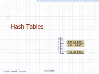
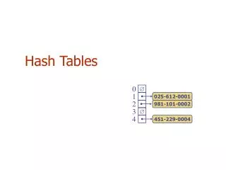
Hash Tables 0 1 025-612-0001 2 981-101-0002 3 4 451-229-0004
Maps and the Map ADT • Mathematically, a Map is a set of ordered pairs whose elements are known as the key and the value • Keys are required to be unique, but values are not necessarily unique • You can think of each key as a “mapping” to a particular value {(J, Jane), (B, Bill), (B2, Bill), (S, Sam), (B1, Bob)}
Map ADT • The main operations of a map are for • searching, • inserting, • and deleting items
Map ADT • Map ADT methods: • get(k): if the map M has an entry with key k, return its assoiciated value; else, return null • put(k, v): insert entry (k, v) into the map M; if key k is not already in M, then return null; else, return old value associated with k • remove(k): if the map M has an entry with key k, remove it from M and return its associated value; else, return null • size(), isEmpty()
Example Operation Output Map isEmpty() true Ø put(5,A) null (5,A) put(7,B) null (5,A),(7,B) put(2,C) null (5,A),(7,B),(2,C) put(8,D) null (5,A),(7,B),(2,C),(8,D) put(2,E) C (5,A),(7,B),(2,E),(8,D) get(7) B (5,A),(7,B),(2,E),(8,D) get(4) null (5,A),(7,B),(2,E),(8,D) get(2) E (5,A),(7,B),(2,E),(8,D) size() 4 (5,A),(7,B),(2,E),(8,D) remove(5) A (7,B),(2,E),(8,D) remove(2) E (7,B),(8,D) get(2) null (7,B),(8,D) isEmpty() false (7,B),(8,D)
Hash Tables • The goal behind the hash table is to be able to access an entry based on its key value, not its location • We want to be able to access an element directly through its key value, rather than having to determine its location first by searching for the key value in the array • Using a hash table enables us to retrieve an item in constant time (on average) linear (worst case)
Index Calculation • The basis of hashing is to transform the item’s key value into an integer value which will then be transformed into a table index • Called a hash function
A hash functionh maps keys of a given type to integers in a fixed interval [0, N- 1] Example:h(x) =x mod Nis a hash function for integer keys The integer h(x) is called the hash value of key x A hash table for a given key type consists of Hash function h Array (called table) of size N When implementing a map with a hash table, the goal is to store item (k, o) at index i=h(k) Hash Functions
0 1 025-612-0001 2 981-101-0002 3 4 451-229-0004 … 9997 9998 200-751-9998 9999 Example • We design a hash table for a map storing entries as (SSN, Name), where SSN (social security number) is a nine-digit positive integer • Our hash table uses an array of sizeN= 10,000 and the hash functionh(x) = last four digits of x
A hash function is usually specified as the composition of two functions: Hash code:h1:keysintegers Compression function:h2: integers [0, N- 1] The hash code is applied first, and the compression function is applied next on the result, i.e., h(x) = h2(h1(x)) The goal of the hash function is to “disperse” the keys in an apparently random way Hash Functions
Methods for Generating Hash Codes • In most applications, the keys will consist of strings of letters or digits rather than a single character • The number of possible key values is much larger than the table size • Generating good hash codes is somewhat of an experimental process • Besides a random distribution of its values, the hash function should be relatively simple and efficient to compute
Memory address: We reinterpret the memory address of the key object as an integer (default hash code of all Java objects) Good in general, except for numeric and string keys Integer cast: We reinterpret the bits of the key as an integer Suitable for keys of length less than or equal to the number of bits of the integer type (e.g., byte, short, int and float in Java) Component sum: We partition the bits of the key into components of fixed length (e.g., 16 or 32 bits) and we sum the components (ignoring overflows) Suitable for numeric keys of fixed length greater than or equal to the number of bits of the integer type (e.g., long and double in Java) Hash Codes
Polynomial accumulation: We partition the bits of the key into a sequence of components of fixed length (e.g., 8, 16 or 32 bits)a0 a1 … an-1 We evaluate the polynomial p(z)= a0+a1 z+a2 z2+ … … +an-1zn-1 at a fixed value z, ignoring overflows Especially suitable for strings (e.g., the choice z =33gives at most 6 collisions on a set of 50,000 English words) Polynomial p(z) can be evaluated in O(n) time using Horner’s rule: The following polynomials are successively computed, each from the previous one in O(1) time p0(z)= an-1 pi(z)= an-i-1 +zpi-1(z) (i =1, 2, …, n -1) We have p(z) = pn-1(z) Hash Codes
Mod: h2 (y) = y mod N The size N of the hash table is usually chosen to be a prime The reason has to do with number theory and is beyond the scope of this course Compression Function
Collisions occur when different elements are mapped to the same cell Separate Chaining: let each cell in the table point to a linked list of entries that map there Separate chaining is simple, but requires additional memory outside the table 0 1 025-612-0001 2 3 4 451-229-0004 981-101-0004 Collision Handling
Open addressing: the colliding item is placed in a different cell of the table Linear probing handles collisions by placing the colliding item in the next (circularly) available table cell Each table cell inspected is referred to as a “probe” Colliding items lump together, causing future collisions to cause a longer sequence of probes Example: h(x) = x mod13 Insert keys 18, 41, 22, 44, 59, 32, 31, 73, in this order Linear Probing 0 1 2 3 4 5 6 7 8 9 10 11 12 41 18 44 59 32 22 31 73 0 1 2 3 4 5 6 7 8 9 10 11 12
Consider a hash table A that uses linear probing get(k) We start at cell h(k) We probe consecutive locations until one of the following occurs An item with key k is found, or An empty cell is found, or N cells have been unsuccessfully probed Search with Linear Probing Algorithmget(k) i h(k) p0 repeat c A[i] if c= returnnull else if c.key () =k returnc.element() else i(i+1)mod N p p+1 untilp=N returnnull
Table Wraparound and Search Termination • As you increment the table index, your table should wrap around as in a circular array • Leads to the potential of an infinite loop • How do you know when to stop searching if the table is full and you have not found the correct value? • Stop when N cells are probed
To handle insertions and deletions, we introduce a special object, called AVAILABLE, which replaces deleted elements remove(k) We search for an entry with key k If such an entry (k, o) is found, we replace it with the special item AVAILABLE and we return element o Else, we return null put(k, o) We throw an exception if the table is full We start at cell h(k) We probe consecutive cells until one of the following occurs A cell i is found that is either empty or stores AVAILABLE, or N cells have been unsuccessfully probed We store entry (k, o) in cell i Updates with Linear Probing
Reducing Collisions Using Quadratic Probing • Linear probing tends to form clusters of keys in the table, causing longer search chains • Quadratic probing can reduce the effect of clustering • For key k, try successively: h(k) mod N, (h(k)+1) mod N, (h(k)+4) mod N, (h(k)+9) mod N, ….
Disadvantages of quadratic probing • Next index calculation is time consuming as it involves multiplication, addition, and modulo division • Not all table elements are examined when looking for an insertion index • cannot insert when table is not full!! • Cannot find an existing item!! • It can be proved that this can’t happen if the table is at most half full, and N is a prime number: but half full table is quite a waste of space.
Let i = h(k) Double hashing uses a secondary hash function d(k) and handles collisions by placing an item in the first available cell of the series (i+jd(k)) mod Nfor j= 0, 1, … , N - 1 The secondary hash function d(k) cannot have zero values The table size N must be a prime to allow probing of all the cells Double Hashing
Double hashing • Common choice for the secondary hash function: • d2(k) = q- k mod q where • q< N • q is a prime • The possible values for d2(k) are 1, 2, … , q
Example of Double Hashing • Consider a hash table storing integer keys that handles collision with double hashing • N= 13 • h(k) = k mod13 • d(k) =7 - k mod7 • Insert keys 18, 41, 22, 44, 59, 32, 31, 73, in this order 0 1 2 3 4 5 6 7 8 9 10 11 12 31 41 18 32 59 73 22 44 0 1 2 3 4 5 6 7 8 9 10 11 12
In the worst case, searches, insertions and removals on a hash table take O(n)time The worst case occurs when all the keys inserted into the map collide The load factor a=n/Naffects the performance of a hash table Assuming that the hash values are like random numbers, it can be shown that the expected number of probes for an insertion with open addressing is1/ (1 -a) The expected running time of all the map ADT operations in a hash table is O(1) In practice, hashing is very fast provided the load factor is not close to 1. Performance of Hashing
Rehash • keep load factor under a desired threshold • Ensure that the table is never full by increasing its size after an insertion if its load factor exceeds a specified threshold • Double the table size • Rehashing all entries to the new table
Implementation Considerations • Class object implements methods hashCode and equals, so every class can access these methods unless it overrides them • Object.equals compares two objects based on their addresses, not their contents • Object.hashCode calculates an object’s hash code based on its address, not its contents • Java recommends that if you override the equals method, then you should also override the hashCode method
Java’s Map based on a HashTable implementation • java.util.HashMap