Efficient Hash Table Implementations and Analysis in Computer Science
230 likes | 252 Vues
Understand the concept, implementation, and analysis of hash tables for insert, search, and delete operations. Learn about direct address tables, hashing functions, collisions, chaining, open addressing, and hash function selection strategies.

Efficient Hash Table Implementations and Analysis in Computer Science
E N D
Presentation Transcript
Hash Tables Chapter 12
Motivation • Many applications require only: • Insert • Search • Delete • Examples • Symbol tables • Memory management mechanisms
Direct-address tables • Assumption- unique keys are taken for a relatively small universe U={0,1,….,m-1} of keys • The set is represented by an array of references (direct access table) T[0..m-1] where entry T[j] may potentially point to an object with key=j
Satellite data T U 2 0 1 3 9 4 8 2 5 3 5 6 7 8
Pseudo-code • directAddressSearch(T,k) return T[k] • directAddressInsert(T,x) T[key(x)]=x • directAddressDelete(T,x) T[key(x)]=null
Hash Tables • In many cases the universe U is large while the set K of keys actually stored is small. • Hash tables are data structures that require a table of size O(|K|) (instead of O(|U|)) only but still provide the O(1) (in average) access time.
Hash function T U
Collisions • A collision occurs when 2 different keys are mapped by h to the same slot in T • how to find hash functions that minimize collisions • Collisions are inevitable • Since |U|>m there must be two keys who have the same value • resolution by chaining • open addressing
Chaining • All the elements that hash to the same slot are kept in a linked list. • chainedHashInsert(T,x) insert x at the head of list T[h(key(x))] • chainedHashSearch(T,k) search for an element with key k in list T[h(k)] • chainedHashDelete(T,x) delete x from the list T[h(key(x))]
Analysis • Assume - n elements are stored in a hash table of size m • load factor • Worst case • If the hash function distributes the elements equally and can be computed in O(1) • average complexity • and if we choose m s.t n=O(m) the average complexity turns into O(1)
Hash Functions • Assume that the keys are natural numbers. • Division method • How to choose m? • powers of 10 and 2 should be avoided (why) • good values for m are prime not to close to powers of 2 • ex- n=2000 m=701
Hash Functions • Multiplication method • choose 0<A<1 • recommended value of A • ex k=123456 m=10000 h(k)=|10000*fract(123456*0.61803)| =|10000*fract(76300.004115)|=|10000*0.004115|=|41.151| =41
Other type of keys • When the keys are not natural numbers we convert them. ex-strings s=“pt” ascii(‘p’) =112, ascii(‘t’)=116 nat(“pt”)= 112*256+116=28788
Open Addressing • All the elements are stored in the table itself (m>n). • When inserting a new element, we successively probe the hash table until we find an empty slot. • The sequence of positions probed should depend on the key inserted (why?)
Open addressing • The hash function is now a function that for each probe provide a slot in the table. • In order to ensure that every hash table position is considered we require probe sequence for every key to be a permutation of 0..m-1
Pseudo Code • openHashInsert(T,x) j=0 k=key(x) repeat z=h(k,j) if T[z]=null or T[z]=Del then T[z]=x return z else j++ until j=m error “table overflow”
Pseudo Code • openHashSearch(T,k) j=0 repeat z=h(k,j) if T[z]<> null and T[z]<>Del and key(T[z])=k then return z else j++ until T[z]=null or j=m return null
Deleting • When deleting we must not replace the element with null (why?) • we use a special Del value to denote that the slot was once used. • openHashDelete(T,x) z = openHashSearch(T,x); if z<>null then T[z]=Del
Hash Functions • We would like the probe sequences distributed equally among the m! possible permutations- Uniform Hashing • Uniform Hashing is difficult to implement • linear probing • quadratic probing • double hashing
Linear Probing • Take an ordinary hash function then • Problem- the sequential quest for empty slots causes primary clustering • long run of occupied slots.
Quadratic Probing • Let h’ be as above: • (mod m) • Adequate constants must be found to ensure that all m slots are probed. • Ex • Suffers from secondary clustering
Double Hashing • The hash function is: • In order to probe all the table h’’(k) must be relatively prime to m. • choose m to be a power of 2 and h’’ to return a odd number • choose m to be prime and h’(k) = k mod m and h’’(k)=1+(k mod m’) where m’ is slightly less than m
Analysis • Assuming a uniform hashing and load factor the average number of probes is at most: • unsuccessful search • successful search