L10. Laser Scanners
L10. Laser Scanners. EECS 598-2: Algorithms for Robotics. Administrative. PS2 is due today PS3 posted later tonight. Last Time. Topological Mapping Key ideas Data Association Nearest Neighbor Joint Compatibility RANSAC. Today. Finish up Data Association Laser scanners


L10. Laser Scanners
E N D
Presentation Transcript
L10. Laser Scanners EECS 598-2: Algorithms for Robotics
Administrative • PS2 is due today • PS3 posted later tonight.
Last Time • Topological Mapping • Key ideas • Data Association • Nearest Neighbor • Joint Compatibility • RANSAC
Today • Finish up Data Association • Laser scanners • Principles of operation, noise characterization • Feature Extraction • Contours • Lines • Split and Fit • Agglomerative Line Fitting • Matching Features
Data Association: NN • Simplest data association scheme: • Nearest neighbor. • We have probabilistic estimates of where our landmarks are • When we get an observation, which landmark does it match “best”? • E.g., use Mahalanobis distance Observation Mahl=1.2 Mahl = 4.2 Landmark 1 Landmark 2
Computing Joint Compatibility • Hypothetical data association • observed three landmarks: • (Nice linear observation model this time) • What is the Mahalanobis distance of the observation with respect to the noisy observation of the RHS? • What is the mean and covariance of the RHS?
RANSAC: Preview • RANdomSAmple Consensus: • Randomly generate models • Test the model. • Pick the best model. • Alternative approach to NN, JCBB • (Typically) non-probabilistic • Can be applied to many problems, not just data association: • Outlier rejection • Line fitting
RANSAC • Idea: If we knew the rigid body transformation that aligned us with the global coordinate frame, NN would work well. • Let’s focus our attention on computing the RBT! • Method: • Randomly pick two landmark pairs, compute the rigid-body transformation that they imply. • Project all observations using that transformation • How many observations have good NN matches to landmarks? • Our “Consensus” Score • Keep the best RBT. (Optional: Refit the RBT based on the consensus set.)
RANSAC • How many random trials do we need? • We have to guess “right” twice in order to get a correct RBT. • Suppose probability of guessing right is p. • Probability of guessing right twice in a row is p2. • If we have 1/p2 trials, we expect to find the right answer about once. • Use K/p2 trials to “make sure we aren’t unlucky”.
RANSAC • Even with small values of ‘p’, we don’t need that many iterations… • a few thousand, maybe. • In some cases, we can exhaustively try all possible combinations. (“exhaustive RANSAC”?)
RANSAC: Discussion • Complexity? • What about higher dimensions/more complex models? • Upsides: • Works well in low-noise/high-ambiguity situations • Allows us to compute a good hypothesis • Very fast in low dimensions • Useful in many contexts: a great general-purpose tool • Easy to incorporate negative information • Downsides: • Not very rigorous • Parameters to tune by hand • What is “close enough” to increase consensus score?
Graph Methods • Most of value of Joint Compatibility can be captured by considering only pairwise compatibility. • Consistency graph • Nodes in the graph are hypotheses (observation i corresponds to landmark j) • Edges represent pairwise consistency • No edge means the two hypotheses are not simultaneously compatible.
Graph Methods: CCDA • Combined Constraint Data Association (CCDA): • Boolean edges (e.g., thresholded Mahalanobis distances) • Find the largest clique in the graph: these are the correct associations. H2 H1 H3 H4 H5 CCDA: H1, H2, H4
Graph Methods: SCGP • Single Cluster Graph Partitioning (SCGP) • Edges have weights (more expressive) • Finds densely-connected subgraph • Doesn’t have to be a clique • Detects ambiguity (two dense subgraphs possible?) • O(N2) H2 H2 H1 H1 H3 H3 H4 H4 H5 H5 CCDA, SCGP: H1, H2, H4 CCDA: ?? SCGP: H1, H2, H4, H5
SCGP sketch • Indicator vector: • Vector of {0,1} which says which nodes to keep • Quantity to maximize: • Differentiate λ with respect to v, obtain: Sum of all pair-wise consistencies between hypotheses in v • vTAv • λ = • vTv Av = λv Number of hypotheses in v
Laser Scanners • Measure range via time-of-flight • SICK • Industrial safety • 180 samples, 1 degree spacing, 75Hz • Resolution ~1cm, ~0.25 deg. • Interlacing • Max range: “80m” 30m fairly reliable • Intensity • $4500 • Hokuyo • ~520 samples, 0.25deg spacing, 15Hz • $2600 - $5000
Aligning Scans = Measuring motion • Two important cases: • Incremental motion. Use lidar to augment (or replace!) odometry. • Loop closing. Identify places we’ve been before to over-constrain robot trajectory.
Feature Extraction • Our plan: • Extract features from two scans • Match features • Compute rigid-body transformation • Possible features: • Lines • Corners • Occlusion boundaries/depth discontinuities • Trees (!)
Line Extraction • Given laser scan, produce a set of 2D line segments • Two basic approaches: • Divisive (“Split N Fit”) • Agglomerative • Our plan: • If we know which points belong to a line, how do we fit a line to those points? • How do we determine which points belong together?
Optimal Line Derivation • Assume we know a set of points belong to a line. How do we compute parameters of the line? • How to parameterize the line? • Slope + y intercept? • Endpoints of line • A point on the line + unit vector • R + theta
Optimal Line Derivation • Error for one point • Cost function • Solution found by minimizing pi e pi-q q, a point on the line θ
Optimal Line Derivation • Method: work in terms of moments:
Optimal Line Derivation • Solution: • Because all quantities are written in terms of moments, we can compute this quantity incrementally and without storing all the points!
Line Fitting: Divisive • Init: All points belong to a single line • Split-N-Fit(points) • Fit line to points • if line error < thresh then • return the line • else • Which point fits the worst? • Split the line into two lines at that point • return Split-N-Fit(leftpoints) U Split-N-Fit(rightpoints)
Line Fitting: Divisive • Pros: • Easy to implement • Cons: • Assumes points are in scan order • Doesn’t always generate good answers • Can split points that should belong together • “Split-N-Fit-N-Merge” • Complexity?
Line Fitting: Agglomerative • Agglomerative-Fit(points) • Init: create N-1 lines for each pair of adjacent points • do forever • for each pair of adjacent lines i, i+1 • Compute error for line that merges those two lines • if minimum error > thresh then • return lines • else • merge lines with minimum error
Line Fitting: Agglomerative • Pros: • Good quality, matches human expectations • Cons: • Assumes points are in scan order • A little bit tricky to implement quickly (use a min-heap) • Complexity?
Line Fitting: RANSAC • Pros: • Easy • Does not require points to be in scan order • Cons: • Hard to exploit points being in scan order • Not obvious how to extract more than one line
Line Fitting: Hough Transform • Each point is evidence for a set of lines • Vote for each of the possible lines. • Lines with lots of evidence get many votes.
Other Features • Corners • Intersections of nearby (?) lines. • Easy to extract from lines. • Only need ONE corner correspondence to compute RBT. • Trees (Victoria Park) • Depth Discontinuities • Beware of viewpoint effects
Contour Extraction • Divisive/Agglomerative line fittings need points to be grouped together • Consider stair railing • Simple agglomerative process works well!
Aligning scans using features • RANSAC! • Randomly guess enough correspondences to fit a model • Pick the model with the best consensus score. • Can incorporate negative information • Penalize consensus if features are missing.
Next Time • Aligning scans without extracting features