Download
1 / 31
310 likes | 496 Vues
LL-III physics-based distributed hydrologic model in Blue River Basin and Baron Fork Basin. Li Lan (State Key Laboratory of Water Resources and Hydropower Engineering Science, Wuhan University, China ,430072). 1. Model Introduction.

E N D
LL-III physics-based distributed hydrologic model in Blue River Basin and Baron Fork Basin Li Lan (State Key Laboratory of Water Resources and Hydropower Engineering Science, Wuhan University, China ,430072)
1. Model Introduction • The LL-I physics-based distributed hydrologic model was produced by Lan Li in Wuhan University in 1997,and in 2002 the LL-II model was put forward based on LL-I when taking part in DMIP-I, then in 2004 the LL-III model was developed.
3. Model Equations • (1)Evaporation 1) Evaporation capacity The plant canopy evapotranspiration is taken Jensen and Haise formula.
Where is the plant canopy evapotranspiration(mms-1), is evaporation of soil, VCF(t) is vegetation cover rate, LAI(t)/LAI0 is relative leaf area index, is available ratio of soil moisture, is soil moisture, is soil porosity, K1 is evapotranspiration coeffition of plant canopy, K2 is evaporation coefficient of soil, is the water vapor density(kg·m-3), L is latent heat of water evaporation(kj·kg-1), is net surface solar radiation, T is temperature (℃), CT is correction factor of the impact that temperature makes on evaporation.
2)The actual soil evaporation rates The equation of actual soil evaporation rates is as follows: And the max evaporation capacity:
Where is diffusivity, is the porosity, is hydraulic conductivity, is a coefficient, is coefficient of recharge by rainfall penetration, is rainfall penetration, is rainfall volume.
(2)Interception Valley interception and effective rainfall is related to vegetation cover and the depth of water accumulation of the basin. Use the following nonlinear formula:
Where is retention coefficient of bare soil • is retention coefficient of vegetation
(3)Infiltration Where is diffusivity, is the porosity, is hydraulic conductivity.
(4) Net rainfall • Where is precipitation, is evaporation, is infiltration, is interception.
(5)Calculation of overland runoff The calculation of overland runoff is based on the convection-diffusion equation derived from shallow water dynamic wave equation and continuous equation, the following forms: Where r stands for precipitation
(6) Subsurface flow • Where: is storativity of aquifer, is unit discharge of subsurface runoff, is actual infiltration rate ( ), is wave velocity of subsurface flow, is outflow coefficient of subsurface flow, is evaporation of soil layer i, is the depth of soil layer i, is infiltration rate of soil layer i, is water death of subsurface soil layer.
(7) Underground runoff • The path of underground runoff is parallel with the overland flow. Underground runoff equation is obtained through continuous equation and the equation of motion:
Where is unit discharge of underground runoff, is wave velocity of underground runoff, is outflow coefficient of undergrou--nd runoff, is the actual infiltration rate when , is evaporation of underground runoff.
(8) Confluence of sub-basin • Reflect the inter-basin links through the boundary conditions • Where is wave velocity, D is Diffusivity, q is unit-width inflow of this sub-basin.
(9) Flow calculation The convergence model uses hydrodynamic equations, continuous equations and momentum equations to calculate the runoff to the space grid nodes of each layer, and uses numerical differential format and numerical analysis to establish relationship of adjacent grid between time and space.
Includes slope convergence and river network convergence. • Slope convergence includes processes of overland flow, subsurface flow, underground runoff etc. • The total of overland flow, subsurface flow, underground runoff is called unit-width inflow. And river network convergence is the convergence process of the unit-width inflow which runs into the river.
4. Parameters calibration • The parameters that need to be determined can be related with the topography parameters, such as DEM, Land cover, NDVI, Soil texture, etc. Only overland flow wave velocity and river wave velocity need to be calibrated by measured data. • The overland flow wave velocity, is the function of Roughness, gradient and strength of net rain.
Parameters calibration • River confluence is the function of Roughness, hydraulic gradient and unit-width flow. • Establish the empirical formulas of interception coefficient and evaporation coefficient according to each month of year 2000 respectively. • And the interception coefficient and is related with effective rainfall (i-E), evaporation coefficient and is related with rainfall strength by calibrated parameters of 2000 year,.
5. Simulation results • 1. Comparison of calculated discharge among the three gauges of Blue River with calibration. See figure 5-1 and figure 5-2. • 2. Comparison of calculated discharge among the three gauges of Baron Fork with calibration. See figure 5-3 and figure 5-4. • 3. Comparison of calculated discharge and observed flow of Blue River. See figure 5-5 and figure 5-6. • 4. Comparison of calculated discharge and observed flow of Baron Fork. See figure 5-7 and figure 5-8.
Figure 5.1 Return
Figure 5-2 Return
Figure 5-3 Return
Figure 5-4 Return
Figure 5-5 Return
Figure 5-6 Return
Figure 5-7 Return
Figure 5-8 Return