Presenting Data
Presenting Data Descriptive Statistics Nominal Level No order, just a name Can report Mode Bar Graph Pie Chart Ordinal Level Rank order only Can Report Mode Median Percentiles Histograms and Pie Charts Interval/Ratio Level Equidistant Can Report Mode, Median, Mean

Presenting Data
E N D
Presentation Transcript
Presenting Data Descriptive Statistics
Nominal Level • No order, just a name • Can report • Mode • Bar Graph • Pie Chart
Ordinal Level • Rank order only • Can Report • Mode • Median • Percentiles • Histograms and Pie Charts
Interval/Ratio Level • Equidistant • Can Report • Mode, Median, Mean • Standard Deviation • Percentiles • Frequency curves, Histograms
Univariate Data • Good to start at the univariate level • Univariate: one variable at a time • Investigate the responses • Assess usability for the rest of the analysis
Frequency Table • Shows how often each response was given by the respondents • Most useful with nominal or ordinal • Interval/ratio has too many categories • In Minitab, Select: Stat>Tables>Tally
Charts and Graphs • Use a bar graph or pie chart if the variable has a limited number of discrete values • Nominal or ordinal measures • Histograms and frequency curves are best for interval/ratio measures • In Minitab, Select: Graph > (and then type)
Normal Curve • The normal curve is critical to assessing normality which is an underlying assumption in inferential statistical procedures • And in reporting of results • Kurtosis: related to the bell-shape • Skewness: symmetry of the curve • If more scores are bunched together on the left side, positive skew (right) • If most scores are bunched together on the right side, negative skew
Normal Curve • To get a statistical summary, including an imposed normal curve in Minitab: • Select: Stat > Basic Statistics > Display Descriptive Statistics > Graph > Graphical Summary
Measures of Central Tendency • Mode: most frequently selected • Bimodal = two modes • If more than two modes, either multiple modes or no mode • Median: halfway point • Not always an actual response • Mean: arithmetic mean
Percentiles • The median is the 50 percentile • A percentile tells you the percentage of responses that fall above and below a particular point • Interquartile range = 75th percentile – 25th percentile • Not affected by outliers as the range is
Z-scores • Standard deviations provide an estimate of variability • If scores follow a ‘normal curve’, you can comparing any two scores by standardizing them • Translate scores into z-scores • (Value – mean) / standard deviation
Statistical Hypotheses • Statistical Hypotheses are statements about population parameters. • Hypotheses are not necessarily true.
In statistics, we test one hypothesis against another… • The hypothesis that we want to prove is called the alternative hypothesis, Ha. • Another hypothesis is formed which contradicts Ha. • This hypothesis is called the null hypothesis, Ho. Ho contains an equality statement.
P-value • The choice of is subjective. • The smaller is, the smaller the critical region. Thus, the harder it is to Reject Ho. • The p-value of a hypothesis test is the smallest value of such that Ho would have been rejected.
Interval Estimates • Statisticians prefer interval estimates. • Something depends on amount of variability in data and how certain we want to be that we are correct. • The degree of certainty that we are correct is known as the level of confidence. • Common levels are 90%, 95%, and 99%.
Statistical Significance • Statistically significant: if the probability of obtaining a statistic by chance is less than the set alpha level (usually 5%)
P-value • The probability, computed assuming that Ho is true, that the test statistic would take a value as extreme or more extreme than that actually observed is called the p-value of the test. • The smaller the p-value, the stronger the evidence against Ho provided by the data. • If the p-value is as small or smaller than alpha, we say that the data are statistically significant at level alpha.
Power • The probability that a fixed level alpha significance test will reject Ho when a particular alternative value of the parameter is true is called the power of the test to detect that alternative. • One way to increase power is to increase sample size.
Use and Abuse • P-values are more informative than the results of a fixed level alpha test. • Beware of placing too much weight on traditional values of alpha. • Very small effects can be highly significant, especially when a test is based on a large sample. • Lack of significance does not imply that Ho is true, especially when the test has low power. • Significance tests are not always valid.