Download

1 / 63
630 likes | 822 Vues
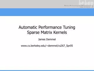
Minimizing Communication in Numerical Linear Algebra www.cs.berkeley.edu/~demmel Sparse-Matrix-Vector-Multiplication ( SpMV ). Jim Demmel EECS & Math Departments, UC Berkeley demmel@cs.berkeley.edu. Outline. Motivation for Automatic Performance Tuning Results for sparse matrix kernels

E N D
Minimizing Communication in Numerical Linear Algebrawww.cs.berkeley.edu/~demmelSparse-Matrix-Vector-Multiplication (SpMV) Jim Demmel EECS & Math Departments, UC Berkeley demmel@cs.berkeley.edu
Outline • Motivation for Automatic Performance Tuning • Results for sparse matrix kernels • Sparse Matrix Vector Multiplication (SpMV) • Sequential and Multicore results • OSKI = Optimized Sparse Kernel Interface • Need to understand tuning of single SpMV to understand opportunities and limits for tuning entire sparse solvers Summer School Lecture 7 2
Berkeley Benchmarking and OPtimization (BeBOP) • Prof. Katherine Yelick • Current members • Kaushik Datta, Mark Hoemmen, Marghoob Mohiyuddin, Shoaib Kamil, Rajesh Nishtala, Vasily Volkov, Sam Williams, … • Previous members • Hormozd Gahvari, Eun-Jim Im, Ankit Jain, Rich Vuduc, many undergrads, … • Many results here from current, previous students • bebop.cs.berkeley.edu Summer School Lecture 7 3
Automatic Performance Tuning • Goal: Let machine do hard work of writing fast code • What does tuning of dense BLAS, FFTs, signal processing, have in common? • Can do the tuning off-line: once per architecture, algorithm • Can take as much time as necessary (hours, a week…) • At run-time, algorithm choice may depend only on few parameters (matrix dimensions, size of FFT, etc.) • Can’t always do tuning off-line • Algorithm and implementation may strongly depend on data only known at run-time • Ex: Sparse matrix nonzero pattern determines both best data structure and implementation of Sparse-matrix-vector-multiplication (SpMV) • Part of search for best algorithm just be done (very quickly!) at run-time Summer School Lecture 7 4
Source: Accelerator Cavity Design Problem (Ko via Husbands) 5
Linear Programming Matrix … Summer School Lecture 7 6
SpMV with Compressed Sparse Row (CSR) Storage Matrix-vector multiply kernel: y(i) y(i) + A(i,j)*x(j) for each row i for k=ptr[i] to ptr[i+1] do y[i] = y[i] + val[k]*x[ind[k]] Matrix-vector multiply kernel: y(i) y(i) + A(i,j)*x(j) for each row i for k=ptr[i] to ptr[i+1] do y[i] = y[i] + val[k]*x[ind[k]] Only 2 flops per 2 mem_refs: Limited by getting data from memory Summer School Lecture 7 8
Example: The Difficulty of Tuning • n = 21200 • nnz = 1.5 M • kernel: SpMV • Source: NASA structural analysis problem 9
Example: The Difficulty of Tuning • n = 21200 • nnz = 1.5 M • kernel: SpMV • Source: NASA structural analysis problem • 8x8 dense substructure: exploit this to limit #mem_refs 10
Taking advantage of block structure in SpMV • Bottleneck is time to get matrix from memory • Only 2 flops for each nonzero in matrix • Don’t store each nonzero with index, instead store each nonzero r-by-c block with index • Storage drops by up to 2x, if rc >> 1, all 32-bit quantities • Time to fetch matrix from memory decreases • Change both data structure and algorithm • Need to pick r and c • Need to change algorithm accordingly • In example, is r=c=8 best choice? • Minimizes storage, so looks like a good idea…
Best: 4x2 Reference Speedups on Itanium 2: The Need for Search Mflop/s Mflop/s 12
Register Profile: Itanium 2 1190 Mflop/s 190 Mflop/s 13
Power3 - 17% Register Profiles: IBM and Intel IA-64 252 Mflop/s Power4 - 16% 820 Mflop/s 122 Mflop/s 459 Mflop/s Itanium 1 - 8% Itanium 2 - 33% 247 Mflop/s 1.2 Gflop/s 107 Mflop/s 190 Mflop/s
Ultra 2i - 11% 72 Mflop/s Ultra 3 - 5% 90 Mflop/s Register Profiles: Sun and Intel x86 35 Mflop/s 50 Mflop/s Pentium III - 21% Pentium III-M - 15% 108 Mflop/s 122 Mflop/s 42 Mflop/s 58 Mflop/s
Another example of tuning challenges • More complicated non-zero structure in general • N = 16614 • NNZ = 1.1M 16
Zoom in to top corner • More complicated non-zero structure in general • N = 16614 • NNZ = 1.1M 17
3x3 blocks look natural, but… • More complicated non-zero structure in general • Example: 3x3 blocking • Logical grid of 3x3 cells • But would lead to lots of “fill-in” 18
Extra Work Can Improve Efficiency! • More complicated non-zero structure in general • Example: 3x3 blocking • Logical grid of 3x3 cells • Fill-in explicit zeros • Unroll 3x3 block multiplies • “Fill ratio” = 1.5 • On Pentium III: 1.5x speedup! • Actual mflop rate 1.52 = 2.25 higher 19
Automatic Register Block Size Selection • Selecting the r x c block size • Off-line benchmark • Precompute Mflops(r,c) using dense A for each r x c • Once per machine/architecture • Run-time “search” • Sample A to estimate Fill(r,c) for each r x c • Run-time heuristic model • Choose r, c to minimize time ~Fill(r,c) /Mflops(r,c) Summer School Lecture 7 20
Accurate and Efficient Adaptive Fill Estimation • Idea: Sample matrix • Fraction of matrix to sample: sÎ [0,1] • Control cost = O(s * nnz ) by controlling s • Search at run-time: the constant matters! • Control s automatically by computing statistical confidence intervals, by monitoring variance • Cost of tuning • Lower bound: convert matrix in 5 to 40 unblocked SpMVs • Heuristic: 1 to 11 SpMVs • Tuning only useful when we do many SpMVs • Common case, eg in sparse solvers 21
Accuracy of the Tuning Heuristics (1/4) See p. 375 of Vuduc’s thesis for matrices NOTE: “Fair” flops used (ops on explicit zeros not counted as “work”) 22
Upper Bounds on Performance for blocked SpMV • P = (flops) / (time) • Flops = 2 * nnz(A) • Upper bound on speed: Two main assumptions • 1. Count memory ops only (streaming) • 2. Count only compulsory, capacity misses: ignore conflicts • Account for line sizes • Account for matrix size and nnz • Charge minimum access “latency” ai at Li cache & amem • e.g., Saavedra-Barrera and PMaC MAPS benchmarks Summer School Lecture 7 25 • Upper bound on time: assume all references to x( ) miss
Summary of Other Performance Optimizations • Optimizations for SpMV • Register blocking (RB): up to 4x over CSR • Variable block splitting: 2.1x over CSR, 1.8x over RB • Diagonals: 2x over CSR • Reordering to create dense structure + splitting: 2x over CSR • Symmetry: 2.8x over CSR, 2.6x over RB • Cache blocking: 2.8x over CSR • Multiple vectors (SpMM): 7x over CSR • And combinations… • Sparse triangular solve • Hybrid sparse/dense data structure: 1.8x over CSR • Higher-level kernels • A·AT·x, AT·A·x: 4x over CSR, 1.8x over RB • A2·x: 2x over CSR, 1.5x over RB • [A·x, A2·x, A3·x, .. , Ak·x] …. more to say later 29
Raefsky4 (structural problem) + SuperLU + colmmd N=19779, nnz=12.6 M Example: Sparse Triangular Factor Dense trailing triangle: dim=2268, 20% of total nz Can be as high as 90+%! 1.8x over CSR 30
“axpy” dot product Cache Optimizations for AAT*x • Cache-level: Interleave multiplication by A, AT • Only fetch A from memory once … … • Register-level: aiT to be r´c block row, or diag row 31
Example: Combining Optimizations (1/2) • Register blocking, symmetry, multiple (k) vectors • Three low-level tuning parameters: r, c, v X k v * r c += Y A 32
Example: Combining Optimizations (2/2) • Register blocking, symmetry, and multiple vectors [Ben Lee @ UCB] • Symmetric, blocked, 1 vector • Up to 2.6x over nonsymmetric, blocked, 1 vector • Symmetric, blocked, k vectors • Up to 2.1x over nonsymmetric, blocked, k vecs. • Up to 7.3x over nonsymmetric, nonblocked, 1, vector • Symmetric Storage: up to 64.7% savings 33
Potential Impact on Applications: Omega3P • Application: accelerator cavity design [Ko] • Relevant optimization techniques • Symmetric storage • Register blocking • Reordering, to create more dense blocks • Reverse Cuthill-McKee ordering to reduce bandwidth • Do Breadth-First-Search, number nodes in reverse order visited • Traveling Salesman Problem-based ordering to create blocks • Nodes = columns of A • Weights(u, v) = no. of nz u, v have in common • Tour = ordering of columns • Choose maximum weight tour • See [Pinar & Heath ’97] • 2.1x speedup on IBM Power 4 34
Source: Accelerator Cavity Design Problem (Ko via Husbands) 35
100x100 Submatrix Along Diagonal Summer School Lecture 7 37
“Microscopic” Effect of RCM Reordering Before: Green + Red After: Green + Blue Summer School Lecture 7 38
“Microscopic” Effect of Combined RCM+TSP Reordering Before: Green + Red After: Green + Blue Summer School Lecture 7 39
(Omega3P) 40
Optimized Sparse Kernel Interface - OSKI • Provides sparse kernels automatically tuned for user’s matrix & machine • BLAS-style functionality: SpMV, Ax & ATy, TrSV • Hides complexity of run-time tuning • Includes new, faster locality-aware kernels: ATAx, Akx • Faster than standard implementations • Up to 4x faster matvec, 1.8x trisolve, 4x ATA*x • For “advanced” users & solver library writers • Available as stand-alone library (OSKI 1.0.1h, 6/07) • Available as PETSc extension (OSKI-PETSc .1d, 3/06) • Bebop.cs.berkeley.edu/oski Summer School Lecture 7 41
How the OSKI Tunes (Overview) Application Run-Time Library Install-Time (offline) 1. Build for Target Arch. 2. Benchmark Workload from program monitoring History Matrix Generated code variants Benchmark data 1. Evaluate Models Heuristic models 2. Select Data Struct. & Code To user: Matrix handle for kernel calls Extensibility: Advanced users may write & dynamically add “Code variants” and “Heuristic models” to system.
How to Call OSKI: Basic Usage • May gradually migrate existing apps • Step 1: “Wrap” existing data structures • Step 2: Make BLAS-like kernel calls int* ptr = …, *ind = …; double* val = …; /* Matrix, in CSR format */ double* x = …, *y = …; /* Let x and y be two dense vectors */ /* Compute y = ·y + ·A·x, 500 times */ for( i = 0; i < 500; i++ ) my_matmult( ptr, ind, val, , x, b, y ); 43
How to Call OSKI: Basic Usage • May gradually migrate existing apps • Step 1: “Wrap” existing data structures • Step 2: Make BLAS-like kernel calls int* ptr = …, *ind = …; double* val = …; /* Matrix, in CSR format */ double* x = …, *y = …; /* Let x and y be two dense vectors */ /*Step 1: Create OSKI wrappers around this data*/ oski_matrix_t A_tunable = oski_CreateMatCSR(ptr, ind, val, num_rows, num_cols, SHARE_INPUTMAT, …); oski_vecview_t x_view = oski_CreateVecView(x, num_cols, UNIT_STRIDE); oski_vecview_t y_view = oski_CreateVecView(y, num_rows, UNIT_STRIDE); /* Compute y = ·y + ·A·x, 500 times */ for( i = 0; i < 500; i++ ) my_matmult( ptr, ind, val, , x, b, y ); 44
How to Call OSKI: Basic Usage • May gradually migrate existing apps • Step 1: “Wrap” existing data structures • Step 2: Make BLAS-like kernel calls int* ptr = …, *ind = …; double* val = …; /* Matrix, in CSR format */ double* x = …, *y = …; /* Let x and y be two dense vectors */ /* Step 1: Create OSKI wrappers around this data */ oski_matrix_t A_tunable = oski_CreateMatCSR(ptr, ind, val, num_rows, num_cols, SHARE_INPUTMAT, …); oski_vecview_t x_view = oski_CreateVecView(x, num_cols, UNIT_STRIDE); oski_vecview_t y_view = oski_CreateVecView(y, num_rows, UNIT_STRIDE); /* Compute y = ·y + ·A·x, 500 times */ for( i = 0; i < 500; i++ ) oski_MatMult(A_tunable, OP_NORMAL, , x_view, , y_view);/* Step 2 */ 45
How to Call OSKI: Tune with Explicit Hints • User calls “tune” routine • May provide explicit tuning hints (OPTIONAL) oski_matrix_t A_tunable = oski_CreateMatCSR( … ); /* … */ /* Tell OSKI we will call SpMV 500 times (workload hint) */ oski_SetHintMatMult(A_tunable, OP_NORMAL, , x_view, , y_view, 500); /* Tell OSKI we think the matrix has 8x8 blocks (structural hint) */ oski_SetHint(A_tunable, HINT_SINGLE_BLOCKSIZE, 8, 8); oski_TuneMat(A_tunable); /* Ask OSKI to tune */ for( i = 0; i < 500; i++ ) oski_MatMult(A_tunable, OP_NORMAL, , x_view, , y_view); 46
How the User Calls OSKI: Implicit Tuning • Ask library to infer workload • Library profiles all kernel calls • May periodically re-tune oski_matrix_t A_tunable = oski_CreateMatCSR( … ); /* … */ for( i = 0; i < 500; i++ ) { oski_MatMult(A_tunable, OP_NORMAL, , x_view, , y_view); oski_TuneMat(A_tunable); /* Ask OSKI to tune */ } Summer School Lecture 7 47
Multicore SMPs Used for Tuning SpMV Intel Xeon E5345 (Clovertown) AMD Opteron 2356 (Barcelona) Sun T2+ T5140 (Victoria Falls) IBM QS20 Cell Blade 48
Multicore SMPs with Conventional cache-based memory hierarchy Intel Xeon E5345 (Clovertown) AMD Opteron 2356 (Barcelona) Sun T2+ T5140 (Victoria Falls) IBM QS20 Cell Blade 49
Multicore SMPs with local store-based memory hierarchy Intel Xeon E5345 (Clovertown) AMD Opteron 2356 (Barcelona) Sun T2+ T5140 (Victoria Falls) IBM QS20 Cell Blade 50