Compressive Signal Processing
DESCRIPTION
Compressive Signal Processing. Richard Baraniuk Rice University. Better, Stronger, Faster. Sense by Sampling. sample. Sense by Sampling. too much data!. sample. Accelerating Data Deluge. 1250 billion gigabytes generated in 2010 # digital bits > # stars in the universe
1 / 0
Télécharger la présentation 

Compressive Signal Processing
An Image/Link below is provided (as is) to download presentation
Download Policy: Content on the Website is provided to you AS IS for your information and personal use and may not be sold / licensed / shared on other websites without getting consent from its author.
Content is provided to you AS IS for your information and personal use only.
Download presentation by click this link.
While downloading, if for some reason you are not able to download a presentation, the publisher may have deleted the file from their server.
During download, if you can't get a presentation, the file might be deleted by the publisher.
E N D
Presentation Transcript
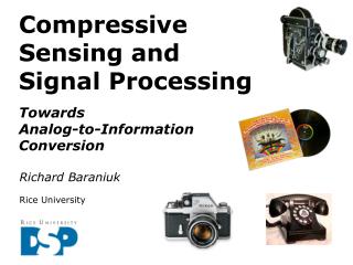
- CompressiveSignal Processing Richard Baraniuk Rice University
- Better, Stronger, Faster
- Sense by Sampling sample
- Sense by Sampling too much data! sample
- Accelerating Data Deluge 1250 billion gigabytes generated in 2010 # digital bits > # stars in the universe growing by a factor of 10 every 5 years Total data generated > total storage Increases in generation rate >>increases in comm rate Available transmission bandwidth
- Sense then Compress sample compress JPEG JPEG2000 … decompress
- Sparsity largewaveletcoefficients (blue = 0) pixels
- Sparsity largewaveletcoefficients (blue = 0) largeGabor (TF)coefficients pixels widebandsignalsamples frequency time
- Concise Signal Structure Sparse signal: only K out of N coordinates nonzero sparsesignal nonzeroentries sorted index
- Concise Signal Structure Sparse signal: only K out of N coordinates nonzero model: union of K-dimensional subspacesaligned w/ coordinate axes sparsesignal nonzeroentries sorted index
- Concise Signal Structure Sparse signal: only K out of N coordinates nonzero model: union of K-dimensional subspaces Compressible signal: sorted coordinates decay rapidly with power-lawapproximately sparse power-lawdecay sorted index
- Concise Signal Structure Sparse signal: only K out of N coordinates nonzero model: union of K-dimensional subspaces Compressible signal: sorted coordinates decay rapidly with power-law model: ball: power-lawdecay sorted index
- What’s Wrong with this Picture? Why go to all the work to acquire N samples only to discard all but K pieces of data? sample compress decompress
- What’s Wrong with this Picture? nonlinear processing nonlinear signal model (union of subspaces) linear processing linear signal model (bandlimited subspace) sample compress decompress
- Compressive Sensing Directly acquire “compressed” data via dimensionality reduction Replace samples by more general “measurements” compressive sensing recover
- Sampling Signal is -sparse in basis/dictionary WLOG assume sparse in space domain sparsesignal nonzeroentries
- Sampling Signal is -sparse in basis/dictionary WLOG assume sparse in space domain Sampling sparsesignal measurements nonzeroentries
- Compressive Sampling When data is sparse/compressible, can directly acquire a condensed representation with no/little information loss through linear dimensionality reduction sparsesignal measurements nonzero entries
- How Can It Work? Projection not full rank…… and so loses information in general Ex: Infinitely many ’s map to the same(null space)
- How Can It Work? Projection not full rank…… and so loses information in general But we are only interested in sparse vectors columns
- How Can It Work? Projection not full rank…… and so loses information in general But we are only interested in sparse vectors is effectively MxK columns
- How Can It Work? Projection not full rank…… and so loses information in general But we are only interested in sparse vectors Design so that each of its MxK submatrices are full rank (ideally close to orthobasis) Restricted Isometry Property (RIP) see also phase transition approach of Donoho et al. columns
- RIP = Stable Embedding An information preserving projection preserves the geometry of the set of sparse signals RIP ensures that K-dim subspaces
- RIP = Stable Embedding An information preserving projection preserves the geometry of the set of sparse signals RIP ensures that
- How Can It Work? Projection not full rank…… and so loses information in general Design so that each of its MxK submatrices are full rank (RIP) Unfortunately, a combinatorial, NP-Hard design problem columns
- Insight from the 70’s [Kashin, Gluskin] Draw at random iid Gaussian iid Bernoulli … Then has the RIP with high probability provided columns
- Randomized Sensing Measurements = random linear combinations of the entries of No information loss for sparse vectors whp sparsesignal measurements nonzero entries
- CS Signal Recovery Goal: Recover signal from measurements Problem: Randomprojection not full rank(ill-posed inverse problem) Solution: Exploit the sparse/compressiblegeometry of acquired signal
- CS Signal Recovery Random projection not full rank Recovery problem:givenfind Null space Search in null space for the “best”according to some criterion ex: least squares (N-M)-dim hyperplaneat random angle
- Signal Recovery Recovery: given(ill-posed inverse problem) find (sparse) Optimization: Closed-form solution:
- Recovery: given(ill-posed inverse problem) find (sparse) Optimization: Closed-form solution: Wrong answer! Signal Recovery
- Recovery: given(ill-posed inverse problem) find (sparse) Optimization: Closed-form solution: Wrong answer! Signal Recovery
- Recovery: given(ill-posed inverse problem) find (sparse) Optimization: Signal Recovery “find sparsest vectorin translated nullspace”
- Recovery: given(ill-posed inverse problem) find (sparse) Optimization: Correct! Signal Recovery “find sparsest vectorin translated nullspace”
- Recovery: given(ill-posed inverse problem) find (sparse) Optimization: Correct! But NP-Complete alg Signal Recovery “find sparsest vectorin translated nullspace”
- Recovery: given(ill-posed inverse problem) find (sparse) Optimization: Convexify the optimization Signal Recovery Donoho Candes Romberg Tao
- Recovery: given(ill-posed inverse problem) find (sparse) Optimization: Convexify the optimization Correct! Polynomial time alg(linear programming) Much recent alg progress greedy, Bayesian approaches, … Signal Recovery
- CS Hallmarks Stable acquisition/recovery process is numerically stable Asymmetrical(most processing at decoder) conventional: smart encoder, dumb decoder CS: dumb encoder, smart decoder Democratic each measurement carries the same amount of information robust to measurement loss and quantization “digital fountain” property Random measurements encrypted Universal same random projections / hardware can be used forany sparse signal class (generic)
- Universality Random measurements can be used for signals sparse in any basis
- Universality Random measurements can be used for signals sparse in any basis
- Universality Random measurements can be used for signals sparse in any basis sparsecoefficient vector nonzero entries
- Compressive SensingIn Action
- “Single-Pixel” CS Camera scene single photon detector imagereconstructionorprocessing DMD DMD random pattern on DMD array w/ Kevin Kelly
- “Single-Pixel” CS Camera scene single photon detector imagereconstructionorprocessing DMD DMD random pattern on DMD array … Flip mirror array M times to acquire M measurements Sparsity-based (linear programming) recovery
- First Image Acquisition target 65536 pixels 1300 measurements (2%) 11000 measurements (16%)
- Utility? Fairchild 100Mpixel CCD single photon detector DMD DMD
- SWIR CS Camera InView “single-pixel” SWIR Camera (1024x768) Target (illuminated in SWIR only) Camera output M = 0.5 N
- CS Hyperspectral Imager (Kevin Kelly Lab, Rice U) spectrometer hyperspectral data cube 450-850nm N=1M space x wavelength voxels M=200k random measurements
- CS-MUVI for Video CS Pendulum speed: 2 sec/cycle Naïve, block-basedL1 recovery of 64x64 video frames for 3 different values of W 1024 2048 4096
- CS-MUVI for Video CS Effective “compression ratio” = 60:1 Low-res preview (32x32) High-res video recovery (128x128) Recovered video (animated)
- Analog-to-Digital Conversion Nyquist rate limits reach of today’s ADCs “Moore’s Law” for ADCs: technology Figure of Merit incorporating sampling rateand dynamic range doubles every 6-8 years Analog-to-Information (A2I) converter wideband signals have high Nyquist rate but are often sparse/compressible develop new ADC technologies to exploit new tradeoffs amongNyquist rate, sampling rate,dynamic range, … frequency hopperspectrogram frequency time
- Random Demodulator
- Sampling Rate Goal: Sample near signal’s (low) “information rate”rather than its (high) Nyquist rate A2Isampling rate number oftones /window Nyquistbandwidth
- Example: Frequency Hopper 20x sub-Nyquist sampling Nyquist rate sampling sparsogram spectrogram
- Example: Frequency Hopper 20x sub-Nyquist sampling Nyquist rate sampling sparsogram spectrogram CS-based AIC conventional ADC 20MHz sampling rate 1MHz sampling rate
- More CS In Action CS makes sense when measurements are expensive Coded imagers x-ray, gamma-ray, IR, THz, … Camera networks sensing/compression/fusion Array processing exploit spatial sparsity of targets Ultrawideband A/D converters exploit sparsity in frequency domain Medical imaging MRI, CT, ultrasound …
- Pros and Cons of Compressive Sensing
- CS – Pro – Measurement Noise Stable recoverywith additive measurement noise Noise is added to Stability: noise only mildly amplified in recovered signal
- CS – Con – Signal Noise Often seek recoverywith additive signal noise Noise is added to Noise folding: signal noise amplified in by 3dB for every doubling of Same effect seen in classical “bandpass subsampling”
- CS – Con – Noise Folding slope = -3 CS recovered signal SNR
- CS – Pro – Dynamic Range As amount of subsampling grows, can employan ADC with a lower sampling rate and hence higher-resolution quantizer
- Dynamic Range Corollary: CS can significantly boost the ENOB of an ADC system for sparse signals CS ADC w/ sparsity conventional ADC
- CS – Pro – Dynamic Range As amount of subsampling grows, can employan ADC with a lower sampling rateand hence higher-resolution quantizer Thus dynamic range of CS ADC can far exceedNyquist ADC With current ADC trends, dynamic range gain is theoretically 7.9dBfor each doubling in
- CS – Pro – Dynamic Range slope = +5 (almost 7.9) dynamic range
- CS – Pro vs. Con SNR: 3dB loss for each doubling of Dynamic Range:up to 7.9dB gain for each doubling of
- Summary: CS Compressive sensing randomized dimensionality reduction exploits signal sparsity information integrates sensing, compression, processing Why it works: with high probability, random projections preserve information in signals with concise geometric structures Enables new sensing architectures cameras, imaging systems, ADCs, radios, arrays, … Important to understand noise-folding/dynamic range trade space
- Open Research Issues Links with information theory new encoding matrix design via codes (LDPC, fountains) new decoding algorithms (BP, AMP, etc.) quantization and rate distortion theory Links with machine learning Johnson-Lindenstrauss, manifold embedding, RIP Processing/inference on random projections filtering, tracking, interference cancellation, … Multi-signal CS array processing, localization, sensor networks, … CS hardware ADCs, receivers, cameras, imagers, arrays, radars, sonars, … 1-bit CS and stable embeddings
- dsp.rice.edu/cs
More Related


