LECTURE 29: TRANSFER FUNCTION REPRESENTATION
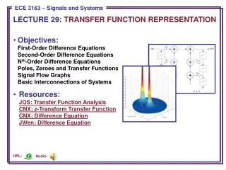
LECTURE 29: TRANSFER FUNCTION REPRESENTATION. Objectives: First-Order Difference Equations Second-Order Difference Equations N th -Order Difference Equations Poles, Zeroes and Transfer Functions Signal Flow Graphs Basic Interconnections of Systems

LECTURE 29: TRANSFER FUNCTION REPRESENTATION
E N D
Presentation Transcript
LECTURE 29: TRANSFER FUNCTION REPRESENTATION • Objectives:First-Order Difference EquationsSecond-Order Difference EquationsNth-Order Difference EquationsPoles, Zeroes and Transfer FunctionsSignal Flow GraphsBasic Interconnections of Systems • Resources:JOS: Transfer Function AnalysisCNX: z-Transform Transfer FunctionCNX: Difference EquationJWen: Difference Equation Audio: URL:
First-Order Difference Equations • Consider a first-order difference equation: • We can apply the time-shift property: • We can solve for Y(z): • The response is again a function of two things: the response due to the initial condition and the response due to the input. • If the initial condition is zero: • Applying the inverse z-Transform: • Is this system causal? Why? • Is this system stable? Why? • Suppose the input was a sinusoid. How would you compute the output?
Example of a First-Order System • Consider the unit-step response of this system: • Use the (1/z) approach for the inverse transform: • The output consists of a DC term, an exponential term due to the I.C., and an exponential term due to the input. Under what conditions is the output stable?
Second-Order Difference Equations • Consider a second-order difference equation: • We can apply the time-shift property: • Assume x[-1] = 0 and solve for Y(z): • Multiplying z2/z2: • Assuming the initial conditions are zero: • Note that the impulse response is of the form: • This can be visualized as a complex pole pair with a center frequency and bandwidth (see Java applet).
Example of a Second-Order System • Consider the unit-step response of this system: • We can further simplify this: • The inverse z-transform gives: MATLAB: num = [1 -1 0]; den = [1 1.5 .5]; n = 0:20; x = ones(1, length(n)); zi = [-1.5*2-0.5*1, -0.5*2]; y = filter(num, den, x, zi);
Nth-Order Difference Equations • Consider a general difference equation: • We can apply the time-shift property once again: • We can again see the important of poles in the stability and overall frequency response of the system. (See Java applet). • Since the coefficients of the denominator are most often real, the transfer function can be factored into a product of complex conjugate poles, which in turn means the impulse response can be computed as the sum of damped sinusoids. Why? • The frequency response of the system can be found by setting z =ej.
Transfer Functions • In addition to our normal transfer function components, such as summation and multiplication, we use one important additional component: delay. • This is often denoted by its z-transform equivalent. • We can illustrate this with an example (assumeinitial conditions are zero): z-1 D
Transfer Function Example • Redraw using z-transform: • Write equations for the behavior at each of the summation nodes: • Three equations and three unknowns: solve the first for Q1(z) and substitute into the other two equations.
Summary • Demonstrated the solution of 1st-order difference equations using thez-transform: general response is an exponential. • Demonstrated the solution of 2nd-order difference equations using thez-transform: general response is a damped sinusoid (complex pole or two real poles). • Discussed the general solution to an Nth-order difference equation: transfer function is a ratio of two polynomials. • Demonstrated how to develop and decompose signal flow graphs using the z-transform: introduced a component, the delay, which is equivalent to differentiation in the s-plane.