Download
1 / 19
190 likes | 216 Vues
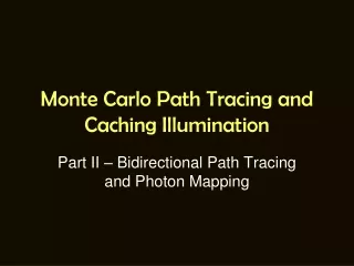
Explore advanced Monte Carlo, path tracing, bi-directional path tracing, and photon mapping for enhanced global illumination in rendering. Learn about vertex connection, photon emission, tracing, storing, radiance estimation, and more. Discover techniques like multiple importance sampling for efficient light transport simulation.

E N D
Monte Carlo Path Tracing and Caching Illumination Part II – Bidirectional Path Tracing and Photon Mapping
Path Notation • A path is written as a regular expression. • Examples: • Ray tracing: LD[S*]E • Radiosity: LD*E • Complete global illumination: L(D|S)*E
Path Tracing • See Pharr’s PBRT 2nd Ed. 15.3
Bi-direction Path Tracing • From Pharr’s PBRT 2nd Ed., Section 15.3.5. • Subpath from camera: p1, p2, …pi • Subpath from light: q1, q2, …qj • The whole path is p1, …, pi, qj, …, q1 • Check if pi can see qj • Some call this “vertex connection”
Bi-direction Path Tracing • Many open questions: • Where does pi or qj end? Does it end on specular or diffuse surfaces? • How to calculate the contribution of qj to pi?
Photon Mapping • See Pharr’s PBRT 2nd Ed., Section 15.6 or SIGGRAPH 2008 Course, Advanced Global Illumination using Photon Mapping
Step 1: Photon Emmision From: SIGGRAPH 2008 Course, Advanced Global Illumination using Photon Mapping Figure 4.1
Step 2: Photon Tracing From: SIGGRAPH 2008 Course, Advanced Global Illumination using Photon Mapping Figure 4.3
Step 3: Photon Storing From: SIGGRAPH 2008 Course, Advanced Global Illumination using Photon Mapping Figure 4.4
Caustic vs. Global Photon Maps From: SIGGRAPH 2008 Course, Advanced Global Illumination using Photon Mapping Figure 4.6
Step 4: Radiance Estimate • Some call this “vertex merging” From: SIGGRAPH 2008 Course, Advanced Global Illumination using Photon Mapping Figure 4.8
Integrals • In rendering equation: • Reflection and transmission. • Visibility • Light source • In image formation (camera) • Pixel • Aperture • Time • Wavelength
Integral of BRDF and Light • Rendering Equation (revisted) • Ignoring emitted light and occlusion, we still have an expensive integral: • Let f(Xi)= (…) I (…) and evaluate its integral with Monte Carlo methods.
Integral of BRDF and Light • Let f(Xi)= (…) I (…) and evaluate its integral. • Case1: a diffuse surface and a few area lights • Case2: a specular surface and environment lighting • Uniform sampling isn’t efficient in both cases. Why? (…) I (…)
Can Importance Sampling Cure Them All? • Consider these two example: • How to handle diffuse reflection? • How to handle large area light source? • More in Veach’s thesis (especially Figure 9.2) • Sampling BRDF vs. sampling light sources
Multiple Importance Sampling • See Pharr’s PBRT 2nd Ed. 14.4 (a) sampling the surface reflectance distribution (b) sampling the area light source
Source: Eric Veach, “Robust Monte Carlo Methods for Light Transport Simulation” Page 255, Figure 9.2. Ph.D. Thesis, Stanford University
References • SIGGRAPH 2008 Course, Advanced Global Illumination using Photon Mapping • SIGGRAPH 2012 Courses, Advanced (quasi) Monte Carlo methods for image synthesis