Path Integral Monte Carlo methods for superfluids

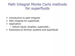
1. Path Integral Monte Carlo methods for superfluids • Introduction to path integrals • Path integrals for superfluids • Application: • Helium liquid, droplets, supersolid,.. • Extensions to fermion systems and superfluids

2. Motivation for Path Integral MC • There are difficulties with VMC and DMC • Need to find good trial functions; this becomes increasing difficult as systems get more complex, especially if one doesn’t know the correct physics. • Mixed estimator problem for properties other than the energy. • Temperature is important: e.g. finite temperature phase transitions. • PIMC makes nice connection with DMC and with other theoretical approaches and leads to concepts such as Reptation MC, understanding of bose condensation, superfluidity, exchange … • Details given in : RMP 67, 279 (1995)

3. Imaginary Time Path Integrals

4. The thermal density matrix • Find exact many-body eigenstates of H. • Probability of occupying state  is exp(-E) • All equilibrium properties can be calculated in terms of thermal o-d density matrix • Convolution theorem relates high temperature to lower temperature.

5. Trotter’s theorem (1959) • We can use the effects of operators separately as long as we take small enough time steps. • n is number of time slices. •  is the “time-step” • We now have to evaluate the density matrix for potential and kinetic matrices by themselves: • Do by FT’s • V is “diagonal” • Error at finite n is roughly: comes from communtator

6. Using this for the density matrix. • We sample the distribution: Where the “primitive” link action is: • Similar to a classical integrand where each particle turns into a “polymer.” • K.E. is spring term holding polymer together. • P.E. is inter-polymer potential. • Trace implies R1=Rm+1 closed or ring polymers

7. “Distinguishable” particles • Each atom is a ring polymer; an exact representation of a quantum wavepacket in imaginary time. • Trace picture of 2D helium. The dots represent the “start” of the path. (but all points are equivalent) • The lower the real temperature, the longer the “string” and the more spread out the wavepacket.

8. Quantum statistics • For quantum many-body problems, not all states are allowed: allowed are totally symmetric or antisymmetric. Statistics are the origin of BEC, superfluidity, lambda transition. • Use permutation operator to project out the correct states: • Means the path closes on itself with a permutation. R1=PRM+1 • Too many permutations to sum over; we must sample them. • PIMC task: sample path { R1,R2,…RM and P} with Metropolis Monte Carlo (MCMC) using “action”, S, to accept/reject.

9. Exchange picture • Average by sampling over all paths and over connections. • Trial moves involve reconnecting paths differently. • At the superfluid transition a “macroscopic” permutation appears. • This is reflection of bose condensation within PIMC.

10. 3 boson example • Suppose the 2 particle action is exact. • Make Jastrow approximation for spatial dependance (Feynman form) • Spatial distribution gives an effective attraction (bose condensation). • For 3 particles we can calculate the “permanent,” but larger systems require us to sample it. • Anyway permutations are more physical.

11. How to choose the action. We don’t have to use the primitive form. Higher order forms cut down on the number of slices by a factor of 10. We can solve the 2-body problem exactly. How to sample the paths and the permutations. Single slice moves are too slow. We move several slices at once. Permutation moves are made by exchanging 2 or more endpoints. How to calculate properties. There are often several ways of calculating properties such as the energy. If you use the simplest algorithm, your code will run 100s or 1000s of times slower than necessary. Calculations of 3000 He atoms can be done on a workstation-- if you are patient. Details see: RMP 67, 279 1995. Main Numerical Issues of PIMC

12. Metropolis Monte Carlo that moves a single variable is too slow and will not generate permutations. We need to move many time slices together Key concept of sampling is how to sample a “bridge”: construct a path starting at R0 and ending at Rt. How do we sample Rt/2? GUIDING RULE. Probability is: Do an entire path by recursion from this formula. Related method: fourier path sampling. PIMC Sampling considerations

13. ß 2. Select permutation from possible pairs, triplets, from: R’ R 0 Bisection method 1. Select time slices 3. Sample midpoints 4. Bisect again, until lowest level 5. Accept or reject entire move

14. Helium phase diagram • Because interaction is so weak helium does not crystallize at low temperatures. Quantum exchange effects are important • Both isotopes are quantum fluids and become superfluids below a critical temperature. • One of the goals of computer simulation is to understand these states, and see how they differ from classical liquids starting from non-relativistic Hamiltonian:

15. Path Integral explanation of Boson superfluidity • Exchange can occur when thermal wavelength is greater than interparticle spacing • Localization in a solid or glass can prevent exchange. • Macroscopic exchange (long permutation cycles) is the underlying phenomena leading to: • Phase transition: bump in specific heat: entropy of long cycles • Superfluiditywinding paths • Offdiagonal long range order--momentum condensationseparation of cut ends • Absence of excitations (gaps) • Some systems exhibit some but not all of these features. • Helium is not the only superfluid. (2001 Nobel Prize for BEC)

16. T=2.5K T=1K Normal “atomic” state “entangled” liquid

17. SPECIFIC HEAT • Characteristic  shape when permutations become macroscopic • Finite size effects cause rounding above transition ENERGY Bose statistics have a small effect on the energy Below 1.5K 4He is in the ground state. Kinetic term becomes smaller because Ncycke<N. Springs stretched more.

18. 4He Superfluidity and PIMC rotating disks: • We define superfluidity as a linear response to a velocity perturbation (the energy needed to rotate the system) “NCRI=nonclassical rotational inertia” • To evaluate with Path Integrals, we use the Hamiltonian in rotating frame: Andronikashvili’s expt (1946) A = signed area of imaginary-time paths

19. Winding numbers in periodic boundary conditions • Distort annulus • The area becomes the winding (average center of mass velocity) • The superfluid density is now estimated as: • Exact linear response formula. (analogous to relation between  ~<M2> for Ising model. • Relates topological property of paths to dynamical response. Explains why superfluid is “protected.” • Imaginary time dynamics is related to real time response. • How the paths are connected is more important than static correlations.

20. Superfluidity in pure Droplets • 64 atom droplet goes into the superfluid state in temperature range 1K <T <2K. NOT A PHASE TRANSITION! • But almost completely superfluid at 0.4K (according to response criteria.) • Superfluidity of small droplets recently verified. Sindzingre et al 1990 Bulk experiment Droplet

21. Droplets and PIMCE. Draeger (LLNL) D. Ceperley(UIUC) • Provide precise microscopic probes for phenomenon such as superfluidity and vortices. • Provide a nearly ideal “spectroscopic matrix” for studying molecular species which may be unstable or weakly interacting in the gas phase. • PIMC can be used to simulate 4He droplets of up to 1000 atoms, at finite temperatures containing impurities, calculating the density distributions, shape deformations and superfluid density. • Droplets are well-suited to take advantage of the strengths of PIMC: • Finite temperature (T=0.38 K) • Bose statistics (no sign problem) • Finite size effects are interesting.

22. Experimental Setupfor He droplets • Adiabatic expansion cools helium to below the critical point, forming droplets. • Droplets then cool by evaporation to: T=0.38 K, (4He) T=0.15 K, (3He) • The droplets are sent through a scattering chamber to pick up impurities, and are detected either with a mass spectrometer with electron-impact ionizer or a bolometer. • Spectroscopy yields the rotational-vibrational spectrum for the impurity to accuracy of 0.01/cm. Almost free rotation in superfluid helium but increase of MOI of rotating impurities. Toennies and Vilesov, Ann. Rev. Phys. Chem. 49, 1 (1998)

23. 4He are “coat” the impurity allowing it to freely rotate in the superfluid they didn’t! How much 4He does it take to “coat” the impurity and get free rotation? Demonstration of droplet superfluidity Grebenev, Toennies, Vilesov: Science 279, 2083 (1998) • An OCS molecule in a 4He droplet shows rotational bands corresponding to free rotation, with an increased moment of inertia (2.7 times higher) • They replaced boson 4He with fermion 3He. If Bose statistics are important, then rotational bands should disappear. • However, commercial 3He has 4He impurities, which would be more strongly attracted to an impurity. • They found that it takes around 60 4He atoms.

24. Small impurities of 4He in 3He 4He 3He 4He is more strongly attracted to impurity because of zero point effects, so it coats the impurity, insulating it from the 3He.

25. Local Superfluid Density Estimator Although superfluid response is a non-local property, we can calculate the local contribution to the total response. Where A is the area. A1 each bead contributes approximation: use only diagonal terms not positive definite could be noisy

26. Local Superfluid Reduction The local superfluid estimator shows a decrease in the superfluid response throughout the first solvation layer. Average over region with cylindrical symmetry T=0.38 K, N=500 (HCN)3

27. Bose condensation • BEC is the macroscopic occupation of a single quantum state (e.g. momentum distribution in the bulk liquid). • The one particle density matrix is defined in terms of open paths: • We cannot calculate n(r,s) on the diagonal. We need one open path, which can then exchange with others. • Condensate fraction is probability of the ends being widely separated versus localized. ODLRO (off-diagonal long range order) (The FT of a constant is a delta function.) • The condensate fraction gives the linear response of the system to another superfluid.

28. How to calculate n(r) • Take diagonal paths and find probability of displacing one end. • advantage: • simultaneous with other averages, • all time slices and particle contribute. • disadvantage: unreliable for r>. 2. Do simulation off the diagonal and measure end-end distribution. Will get condensate when free end hooks onto a long exchange. • advantage: works for any r • Disadvantage: • Offdiagonal simulation not good for other properties • Normalization problem.

29. Comparison with experiment Single particle density matrix Condensate fraction Neutron scattering cross section

30. Surface of Liquid Helium2 possible pictures of the surface • Dilute Bose gas model:Griffin and Stringari, PRL 76, 259 (1996). • Ripplon model: Galli and Reatto, J. Phys. CM 12,6009 (2000). bulk: n0 = 9% 4He surface: n0 = 100% Can smeared density profile be caused by ripplons alone? Density profile does not distinguish 4He surface: n0 = 50%

31. Condensate Fraction at the Surface of 4He • PIMC supports dilute gas model. • Jastrow wavefunction • Shadow wavefunction

32. Dictionary of the Quantum-Classical Isomorphism Properties of a quantum system are mapped into properties of the fictitious polymer system Attention: some words have opposite meanings.

33. “Direct” Fermion Path Integrals • Path integrals map quantum mechanics into a system of cross-linking closed “polymers.” R0=PRM, P permutation, S(Ri, Ri+1) is “boltzmannon action” • Bosons are easy: simply sample P. • Fermions: sample the “action” and carry (-1)Pas a weight. • Observable is even P - odd P. scales exponentially in N and T-1! 4 quantum paths

34. To get around the sign problem, why not just use the fixed-node method? What nodes? The ground state nodes are not necessarily the correct ones at T>>0. The nodes of the density matrix have an imaginary time dependence. High temperature Low temperature

35. Fixed-Node method with PIMC • Get rid of negative walks by canceling them with positive walks. We can do this if we know where the density matrix changes sign. Restrict walks to those that stay on the same side of the node. • Fixed-node identity. Gives exact solution if we know the places where the density matrix changes sign: the nodes. • Classical correspondence exists!! • Problem: fermion density matrix appears on both sides of the equation. We need nodes to find the density matrix. • But still useful approach. (In classical world we don’t know V(R).)

36.  R0 PR0 R Proof of the fixed node method • The density matrix satisfies the Bloch equation with initial conditions. • One can use more general boundary conditions, not only initial conditions, because solution at the interior is uniquely determined by the exterior-just like the equivalent electrostatic problem. • Suppose someone told us the surfaces where the density matrix vanishes (the nodes). Use them as boundary conditions. • Putting an infinite repulsive potential at the barrier will enforce the boundary condition. • Returning to PI’s, any walk trying to cross the nodes will be killed. • This means that we just restrict path integrals to stay in one region. pos neg neg

37. Ortho-para H2 example In many-body systems it is hard to visualize statistics. • The simplest example of the effect of statistics is the H2 molecule in electronic ground state. • Protons are fermions-must be antisymmetric. • Spins symmetric (). spatial wf antisymmetric (ortho) “fermions” • Spins antisymmetric (- ). spatial wf symmetic (para) “bosons” • Non symmetrical case (HD) “boltzmannons” All 3 cases appear in nature! • Go to relative coordinates: r= r1-r2 • Assume the bond length is fixed |r|=a. Paths are on surface of sphere of radius a. PIMC task is to integrate over such paths with given symmetries. For a single molecule there is no potential term, a “ring polymer” trapped on the surface of a sphere.

38. Paths on a sphere • “boltzmannons”Ring polymers on sphere O(r r) • “bosons” 2 types of paths allowed. O(r  r) + O(r  -r) • ”fermions” 2 types of paths allowed O(r  r) - O(r  -r) Low efficiency as 

39. Restricted paths for ortho H2 • Fix origin of path: the reference point. • Only allow points on path with a positive density matrix. paths staying in the northern hemisphere: r(t).r(0)>0 • Clearly negative paths are thrown out. • They have cancelled against positive paths which went south and then came back north to close. • The symmetrical rule in “t”: r(t).r(t’)>0 is incorrect. • Spherical symmetry is restored by averaging over the reference point: the north pole can be anywhere. • Can do many H2 the same way. • Ortho H2 is much more orientable than either HD or para H2.

40. RPIMC with approximate nodes • In almost all cases, we do not know the “nodal” surfaces. • We must make an an ansatz. • This means we get a fermion density matrix (function with the right symmetry) which satisfies the Bloch equation at all points except at the node. • That is, it has all the exact “bosonic” correlation • There will be a derivative mismatch across the nodal surface unless nodes are correct. • In many cases, there is a free energy bound. (proved at high temperature and at zero temperature and when energy is always lower.) • Maybe one can find the best nodes using the variational principle. (variational density matrix approach)

41. Exciton superfluidity • What system is the most appropriate to observe superfluidity of fermions? (strongest pairing) • Consider the simplest 1-band model of particles and holes in a semiconductor. • Assume masses are isotropic and the same; only the charge is different. • At low temperature a particle and hole can bind together to form an exciton (like a hydrogen atom) which is a boson. • If the exciton density is high enough, they can bose condense.: T3/2<2.7 • Shumway-Ceperley (1999) observed this transition for excitons. • What do the paths look like? • Observed in Oct 2003 in atom traps! BCS region

42. Pairing Nodes • Free fermion nodes does not allow pairing because nodes of two species are independent. • Consider two pairs of fermions. • Possible exchanges are {I, PaPb} and {Pa , Pb}. • The permutationPaPb represents an exciton exchange but it is forbidden if nodes are independent since the path will cross “a” nodes or “b” nodes first. • Instead we used paired nodes: A{ g(a1-b1)g(a2-b2)…..} where g(r) is a pairing function (we used a Gaussian). • Nodes are time-independent  winding number formula for superfluid response. • We can define 2 different responses. Let Wx be winding number of species x. • movement of walls: <(Wa+Wb)2> • magnetic field: <(Wa-Wb)2>

43. BEC of excitons [rs=6 T<Tc] Pair exchange (2,2) Winding exchange (3,6) Blue=electron lavendar=hole Superconductivity is (cooper pairing) of paths.

44. TheoreticalPractical • Restricted paths allow realistic calculations of many fermion systems. No sign problem. • Generalization of bosonic PIMC. • Unifies theory of bose and fermi systems: ring exchanges important for both. • Makes a nodal assumption which is only controlled for T>TF • No Born-Oppenheimer approximation • Fully quantum protons • No density functional needed • No pseudopotential/k-space cutoff • No empirical potentials/chemical model • Paths get stuck at low temperature T<0.1 TF unless you make other assumptions (e.g. ground state nodes.) • CEIMC allows lower temperature PI simulations.