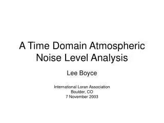
A Time Domain Atmospheric Noise Level Analysis
930 likes | 1.11k Vues
A Time Domain Atmospheric Noise Level Analysis. Lee Boyce International Loran Association Boulder, CO 7 November 2003. Lightning. Cloud to Ground Preliminary breakdown Stepped leader Attachment First return stroke J & K process Dart leader Subsequent return stroke

A Time Domain Atmospheric Noise Level Analysis
E N D
Presentation Transcript
A Time Domain Atmospheric Noise Level Analysis Lee Boyce International Loran Association Boulder, CO 7 November 2003
Lightning • Cloud to Ground • Preliminary breakdown • Stepped leader • Attachment • First return stroke • J & K process • Dart leader • Subsequent return stroke • Intra-Cloud Discharge • J & K process • Q noise
Time Histories Return Preliminary Breakdown Stepped Leader Unipolar & Bipolar K-Process ~400us
Clipping and Hole-Punching Clipping Unfiltered Hole-Punching (Blanking)
Key Question • How do we claim credit for hole-punching over linear processing? • Past work • Feldman 12dB-17dB improvement (on severe days) using two channels for a communication receiver. • Spaulding & Middleton LOBD 30dB, but there are many caveats. • Qualitative explanation • Usually performance will be a function of the level at which the Non-Gaussian component takes over. • Can come up with an estimate based on “hole-punching” that is not too bad.
Goals • Calculate a bound for noise analysis that is better than linear processing • Use available data (CCIR, measurements) • Hole-punch out large nonGaussian impulses • Calculate Gaussian residual • Develop a model for atmospheric noise
CCIR • Used the ARN-2 Radio Noise Recorder • 16 Stations around the globe • Average noise power at each of eight frequencies for fifteen minutes each hour • 13 kHz, 11kHz, 250kHz, 500kHz, 2.5MHz, 5MHz, 10MHz, and 20MHz • 1957-1961 (4 years) → 8640 15-minute measurements → 99.98% • Tracked filtered noise envelope not instantaneous noise • Took high speed data to obtain APDs (400Hz) • Sectioned the year into seasons and time blocks • Four 90-day seasons • Six 4-hour time blocks • Tracked external antenna noise factor, Fa • Power received through a loss-free antenna Fa = 10*log10(Pn/KToB) • Lists the median value hourly value for each time block, Fam, at 1 MHz • Lists the upper decile (90%) level Du • Calculate noise E-field from Fa, BW, frequency • Use normal or log-normal statistics and graphs to adjust values • Limitations • Average background noise, local thunderstorms not included • If power averaged over several minutes, it’s a constant, except when there are local thunderstorms • Noise BW is wider than Rx BW
CCIR (cont) • Noise Factor, Fa • Determines absolute measure Erms (uV/m) • Varies with location • Bandwidth independent • Voltage deviation, Vd • Determines APD curve • Uncorrelated to Noise Factor • APD gives strength relative to RMS value, parameterized by Vd • Enoise(%) = Erms(Fa) + APD(Vd)
APD Review • Amplitude Probability Distributions or Apriori Probability Distributions • APD = 1 - CDF • Shows the percentage of time that a given envelope voltage level is exceeded • Envelope, A, is Rayleigh = Sqrt(Gaussian12 + Gaussian22) • Rayleigh Distribution is a Line • Values relative to RMS (0 dB) • Parameterized by Voltage Deviation, Vd • Vd = 20*log10(RMS Voltage / Avg Voltage) • High amplitude samples dominate Vd D = A - Arms 0 0.0001% 36% 99% P [D Exceeded]
60 50 40 30 20 10 0 -10 -20 -30 -40 • CCIR uses these • Large database over 4 years • APD referenced to RMS value • Parameterized by Vd • Noise BW is wider than Rx 0dB = ARMS D = A - Arms Vd = 1.05 Vd=30 12 14 0.01 1 5 10 20 30 40 50 60 70 80 85 90 95 98 99 0.001 0.1 P [D Exceeded] 0.0001
60 50 40 30 20 10 0 -10 -20 -30 -40 • Atmospheric noise is Non-Gaussian overall but has a strong Gaussian component, hence Rayleigh Envelope • Vd coupled amount of time that the signal is Rayleigh • Hole Punch whenever the Noise Level is more than 3dB above the Rayleigh component • Get measure of signal suppression D = A - Arms Rayleigh Vd = 1.05 3dB Hole Punched “Suppressed” Vd = 10 Rayleigh “Available” 0.01 1 5 10 20 30 40 50 60 70 80 85 90 95 98 99 0.001 0.1 P [D Exceeded] 0.0001
Hole Punch Signal Suppression Loss or Signal Suppression [dB]
60 50 40 30 20 10 0 -10 -20 -30 -40 • Vd coupled to the strength of Rayleigh Component • Measured how far below RMS value Rayleigh component was • Get measure of Rayleigh signal strength • Reduces the noise numbers D = A - Arms Rayleigh Level Relative to RMS Rayleigh -20dB Vd = 1.05 Vd = 10 0.01 1 5 10 20 30 40 50 60 70 80 85 90 95 98 99 0.001 0.1 P [D Exceeded] 0.0001
Noise Model • Break up Atmospheric Noise into two parts • Hole Punch non-Rayleigh (nonGaussian) noise out • Increases Noise • Reduce noise level from RMS value to Rayleigh level • Decreases Noise
Summary of Noise 1 Summer 18h Worst Case 2 Spring 18h Worst Case
July 9, 2002 Upland, IN>10kA Strikes 1600-2259 UTC (10:00a – 4:59p CDT) Click on map for animation
Taylor Univ. - Upland, Indiana • 300Hz-40kHz BW • 100kS/s • Filter BW wide enough to contain interference
Results of Processing • Less signal suppression than predicted • Lower difference between Vrms and Rayleigh Level • Median 50% E-field @ Taylor 20kHz BW 40kHz = 75 dB uV/m
Simulation • Try to keep 1st Order Statistics (APD) • Get the flavor of the time structure • Use two continuous Markov processes to describe close and far discharges
Markov Chain for Discharges Local Remote
Data Comparison Data Simulation
Summary • Non-linear processing analysis should give goals for real design. • Have the makings of a good atmospheric noise model. • 1st order statistics preserved • Adequately show time dependency • Need data from Midwest or Gulf during peak times with Loran Rx to verify analysis.
Acknowledgements • Mitch Narins FAA Program Manager • John Cramer & Ken Cummins, Vaisala Inc • Umran Inan & Troy Wood, Department of Electrical Engineering, Stanford University
What is the correct N in SNR? • Need to estimate the noise and the processing gains correctly. • Frequency domain estimate will kill us. • Is there structure in the time domain that we may exploit? • Model as Gaussian + impulsive noise? 110 90 70 50 30 10 -10 -30 E-Field (dB uV/m) Courtesy of Weidman et al 1981
Sept 2001 Data Night Day High Activity Low Activity +22dB to Noise and +15dB to Vd due to BWR