Recap
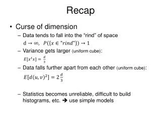
Recap. Curse of dimension Data tends to fall into the “rind” of space Variance gets larger (uniform cube) : Data falls further apart from each other (uniform cube ) : Statistics becomes unreliable, difficult to build histograms, etc. use simple models. Recap. Multivariate Gaussian

Recap
E N D
Presentation Transcript
Recap • Curse of dimension • Data tends to fall into the “rind” of space • Variance gets larger (uniform cube): • Data falls further apart from each other (uniform cube): • Statistics becomes unreliable, difficult to build histograms, etc. use simple models
Recap • Multivariate Gaussian • By translation and rotation, it turns into multiplication of normal distributions • MLE of mean: • MLE of covariance:
Be cautious.. Data may not be in one blob, need to separate data into groups Clustering
CS 498 Probability & Statistics Clustering methods Zicheng Liao
What is clustering? • “Grouping” • A fundamental part in signal processing • “Unsupervised classification” • Assign the same label to data points that are close to each other Why?
Two (types of) clustering methods • Agglomerative/Divisive clustering • K-means
Agglomerative/Divisive clustering Agglomerative clustering Divisive clustering Hierarchical cluster tree (Bottom up) (Top down)
Agglomerative clustering: an example • “merge clusters bottom up to form a hierarchical cluster tree” Animation from Georg Berber www.mit.edu/~georg/papers/lecture6.ppt
Dendrogram Distance >> X = rand(6, 2); %create 6 points on a plane >> Z = linkage(X); %Z encodes a tree of hierarchical clusters >> dendrogram(Z); %visualize Z as a dendrograph
Distance measure • Popular choices:Euclidean, hamming, correlation, cosine,… • A metric • (triangle inequality) • Critical to clustering performance • No single answer, depends on the data and the goal • Data whitening when we know little about the data
Inter-cluster distance • Treat each data point as a single cluster • Only need to define inter-cluster distance • Distance between one set of points and another set of points • 3 popular inter-cluster distances • Single-link • Complete-link • Averaged-link
Single-link • Minimum of all pairwise distances between points from two clusters • Tend to produce long, loose clusters
Complete-link • Maximum of all pairwise distances between points from two clusters • Tend to produce tight clusters
Averaged-link • Average of all pairwise distances between points from two clusters
How many clusters are there? • Intrinsically hard to know • The dendrogram gives insights to it • Choose a threshold to split the dendrogram into clusters Distance
An example do_agglomerative.m
Divisive clustering • “recursively split a cluster into smaller clusters” • It’s hard to choose where to split: combinatorial problem • Can be easier when data has a special structure (pixel grid)
K-means • Partition data into clusters such that: • Clusters are tight (distance to cluster center is small) • Every data point is closer to its own cluster center than to all other cluster centers (Voronoi diagram) [figures excerpted from Wikipedia]
Formulation • Find K clusters that minimize: • Two parameters: • NP-hard for global optimal solution • Iterative procedure (local minimum) Cluster center
K-means algorithm • Choose cluster number K • Initialize cluster center • Randomly select K data points as cluster centers • Randomly assign data to clusters, compute the cluster center • Iterate: • Assign each point to the closest cluster center • Update cluster centers (take the mean of data in each cluster) • Stop when the assignment doesn’t change
Illustration Randomly initialize 3 cluster centers (circles) Assign each point to the closest cluster center Update cluster center Re-iterate step2 [figures excerpted from Wikipedia]
Example do_Kmeans.m (show step-by-step updates and effects of cluster number)
Discussion • How to choose cluster number ? • No exact answer, guess from data (with visualization) • Define a cluster quality measure then optimize K = 2? K = 3? K = 5?
Discussion • Converge to local minimum => counterintuitive clustering 1 2 3 6 5 4 [figures excerpted from Wikipedia]
Discussion • Favors spherical clusters; • Poor results for long/loose/stretched clusters Input data(color indicates true labels) K-means results
Discussion • Cost is guaranteed to decrease in every step • Assign a point to the closest cluster center minimizes the cost for current cluster center configuration • Choose the mean of each cluster as new cluster center minimizes the squared distance for current clustering configuration • Finish in polynomial time
Summary • Clustering as grouping “similar” data together • A world full of clusters/patterns • Two algorithms • Agglomerative/divisive clustering: hierarchical clustering tree • K-means: vector quantization
CS 498 Probability & Statistics Regression Zicheng Liao
Example-I • Predict stock price Stock price t+1 time
Example-II • Fill in missing pixels in an image: inpainting
Example-III • Discover relationship in data Time in service for devices from 3 production lots Amount of hormones by devices from 3 production lots
Example-III • Discovery relationship in data
Linear regression • Input: • Linear model with Gaussian noise • : explanatory variable • : dependent variable • : parameter of linear model • : zero mean Gaussian random variable
Parameter estimation • MLE of linear model with Gaussian noise Likelihood function [Least squares, Carl F. Gauss, 1809]
Parameter estimation • Closed form solution Cost function Normal equation (expensive to compute the matrix inverse for high dimension)
Gradient descent • http://openclassroom.stanford.edu/MainFolder/VideoPage.php?course=MachineLearning&video=02.5-LinearRegressionI-GradientDescentForLinearRegression&speed=100(Andrew Ng) Init: Repeat: Until converge. (Guarantees to reach global minimum in finite steps)
Example do_regression.m
Interpreting a regression • Zero mean residual • Zero correlation
Interpreting the residual • has zero mean • is orthogonal to every column of • is also de-correlated from every column of • is orthogonal to the regression vector • is also de-correlatedfrom the regression vector (follow the same line of derivation)
How good is a fit? • Information ~ variance • Total variance is decoupled into regression variance and error variance • How good is a fit: How much variance is explained by regression: (Because and have zero covariance)
How good is a fit? • R-squared measure • The percentage of variance explained by regression • Used in hypothesis test for model selection
Regularized linear regression • Cost • Closed-form solution • Gradient descent Penalize large values in Init: Repeat: Until converge.
Why regularization? • Handle small eigenvalues • Avoid dividing by small values by adding the regularizer
Why regularization? • Avoid over-fitting: • Over fitting • Small parameters simpler model less prone to over-fitting Smaller parameters make a simpler (better) model Over fit: hard to generalize to new data
L1 regularization (Lasso) • Some features may be irrelevant but still have a small non-zero coefficient in • L1 regularization pushes small values of to zero • “Sparse representation”
How does it work? • When is small, the L1 penalty is much larger than squared penalty. • Causes trouble in optimization (gradient non-continuity)