Chapter 9 Code optimization Section 0 overview
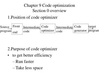
Front end. target program. Code optimizer. Code generator. Source program. Intermediate code. Intermediate code. Chapter 9 Code optimization Section 0 overview. 1.Position of code optimizer 2.Purpose of code optimizer to get better efficiency Run faster Take less space.

Chapter 9 Code optimization Section 0 overview
E N D
Presentation Transcript
Front end target program Code optimizer Code generator Source program Intermediate code Intermediate code Chapter 9 Code optimization Section 0 overview 1.Position of code optimizer 2.Purpose of code optimizer • to get better efficiency • Run faster • Take less space
Chapter 9 Code optimization Section 0 Overview 3. Places for potential improvements by the user and the compiler • Source code • User can profile program,change algorithm or transform loops. • Intermediate code • Compiler can improve loops, procedure calls or address calculations • Target code • Compiler can use registers, select instructions or do peephole transformations
Chapter 9 Code optimization Section 0 overview 4. An organization for an optimizing compiler 1) we assume that the intermediate code consists of three-address statements. 2) organization of the code optimizer Control-flow analysis Data-flow analysis transformations
Chapter 9 Code optimization Section 0 overview 5. Control-flow analysis • Identify blocks and loops in the flow graph of a program 6. Data-flow analysis • Collect information about the program as a whole and to distribute this information to each block in the flow graph.
Chapter 9 Code optimization Section 1 Basic Blocks and flow graphs 1.Flow graph • A directed graph that are composed of the set of basic blocks making up a program
Chapter 9 Code optimization Section 1 Basic Blocks and flow graphs 2.Basic blocks • A sequence of consecutive statements in which flow of control enters at the beginning and leaves at the end without halt or possibility of branching except at the end.
E.g. this is a basic block T1=a*a T2=a*b T3=2*T2 T4=T1+T3 T5=b*b T6=T4+T5 Notes: A name in a basic block is said to be live at a given point if its value is used after that point in the program, perhaps in another basic block.
Chapter 9 Code optimization Section 1 Basic Blocks and flow graphs 3.Partition into basic blocks • Input. A sequence of three-address statements • Output. A list of basic blocks with each three-address statement in exactly one block. • Method. 1) We first determine the set of leaders, the first statements of basic blocks.The rules we use are the following:
Chapter 9 Code optimization Section 1 Basic Blocks and flow graphs 2.Partition into basic blocks • We first determine the set of leaders.The rules : • (1) The first statement is a leader. • (2) Any statement that is the target of a conditional or unconditional goto is a leader. • (3) Any statement that immediately follows a goto or conditional goto statement is a leader.
Chapter 9 Code optimization Section 1 Basic Blocks and flow graphs 2.Partition into basic blocks 2) For each leader, its basic block consists of the leader and all statements up to but not including the next leader or the end of the program.
e.g. begin read X; read Y; while (X mod Y<>0) do begin T:=X mod Y; X:=Y; Y:=T end; write Y end (1)Read X (2)Read Y (3) T1:=X mod Y (4) If T1<>0 goto (6) (5)goto (10) (6)T:=X mod Y (7)X:=Y (8)Y:=T (9)goto (3) (10)write Y (11)halt
(1)Read X (2)Read Y (3) T1:=X mod Y (4) If T1<>0 goto (6) (5)goto (10) (6)T:=X mod Y (7)X:=Y (8)Y:=T (9)goto (3) (10)write Y (11)halt
Chapter 9 Code optimization Section 2 Optimization of basic blocks 1.Function-preserving transformations 1)Methods • Constant folding • The evaluation at compile-time of expressions whose operands are known to be constant • Common sub-expression elimination • Copy propagation • Dead-code elimination
Chapter 9 Code optimization Section 2 Optimization of basic blocks 1.Function-preserving transformations 2)Constant folding & Common sub-expression elimination • An expression E is called a common sub-expression if an expression E was previously computed, and the values of variables in E have not changed since the previous computation. Notes: We can avoid re-computing the expression if we can use the previously computed value
e.g:A source code Pi:=3.14 A:=2*Pi*(R+r); B:=A; B:=2* Pi*(R+r)*(R-r) (1)Pi:=3.14 (2)T1:=2*Pi (3)T2:=R+r (4)A:=T1*T2 (5)B:=A (6)T3:=2*Pi (7)T4:=R+r (8)T5:=T3*T4 (9)T6:=R-r (10)B:=T5*T6
(1)Pi:=3.14 (2)T1:=6.28 (3)T2:=R+r (4)A:=T1*T2 (5)B:=A (6)T3:=6.28 (7)T4:=R+r (8)T5:=T3*T4 (9)T6:=R-r (10)B:=T5*T6 (1)Pi:=3.14 (2)T1:=6.28 (3)T2:=R+r (4)A:=T1*T2 (5)B:=A (6)T3:=T1 (7)T4:=T2 (8)T5:=T3*T4 (9)T6:=R-r (10)B:=T5*T6
Chapter 9 Code optimization Section 2 Optimization of basic blocks 1.Function-preserving transformations 3)Copy Propagation • One concerns assignments of the form f:=g called copy statements
(1)Pi:=3.14 (2)T1:=6.28 (3)T2:=R+r (4)A:=T1*T2 (5)B:=A (6)T3:=T1 (7)T4:=T2 (8)T5:=T1*T2 (9)T6:=R-r (10)B:=T5*T6 (1)Pi:=3.14 (2)T1:=6.28 (3)T2:=R+r (4)A:=T1*T2 (5)B:=A (6)T3:=T1 (7)T4:=T2 (8)T5:=T3*T4 (9)T6:=R-r (10)B:=T5*T6
Chapter 9 Code optimization Section 2 Optimization of basic blocks 1.Function-preserving transformations 4) Dead-code elimination • A variable is live at a point in a program if its value can be used subsequently; otherwise it is dead at that point. Notes: A related idea is dead or useless code, statements that compute values that never get used.
(1)Pi:=3.14 (2)T1:=6.28 (3)T2:=R+r (4)A:=T1*T2 (5)B:=A (6)T3:=T1 (7)T4:=T2 (8)T5:=T1*T2 (9)T6:=R-r (10)B:=T5*T6 (1)Pi:=3.14 (2)T1:=6.28 (3)T2:=R+r (4)A:=T1*T2 (8)T5:=T1*T2 (9)T6:=R-r (10)B:=T5*T6
Chapter 9 Code optimization Section 2 Optimization of basic blocks 2.DAG • There is a node in the dag for each of the initial values of the variables appearing in the basic block. • There is a node n associated with each statement s within the block. • The children of n are those nodes corresponding to statements that are the last definitions prior to s of the operands used by s.
Chapter 9 Code optimization Section 2 Optimization of basic blocks 2.DAG • Node n is labeled by the operator applied at s, and also attached to n is the list of variables for which it is the last definition within the block.
A A (s) n3 n3 n3 rop =[] op A n2 n4 n1 n1 n1 n2 n2 n2 op []= C C C B B B n1 n1 n2 n3 B D C B
B n5 * A,D n3 + n1 n2 n4 C 2 B e.g. A:=B+C B:=2*A D:=A
e.g. (1)T0:=3.14 (2)T1:=2*T0 (3)T2:=R+r (4)A:=T1*T2 (5)B:=A (6)T3:=2*T0 (7)T4:=R+r (8)T5:=T3*T4 (9)T6:=R-r (10)B:=T5*T6
n8 B * n6 A,T5 * n5 T2,T4 n7 - + n3 n4 T1,T3 n1 T0 n2 r R 6.28 3.14 n8 B * n6 A * n5 n7 S2 S1 - + n3 n4 n2 r R 6.28
t4 - t3 - t1 + t2 + A0 b0 e0 C0 d0 Chapter 9 Code optimization Section 2 Optimization of basic blocks 3.Generating code from dags • Rearranging the order(Heuristic Order) T1=a+b T2=c+d T3=e-t2 T4=t1-t3 T2=c+d T3=e-t2 T1=a+b T4=t1-t3
Chapter 9 Code optimization Section 2 Optimization of basic blocks 3.Generating code from dags • Heuristic Order while (unlisted interior nodes remain) { select an unlisted node n, all of whose parents have been listed; list n; while (the leftmost child m of n has no unlisted parents and is not a leaf) { list m; n=m} }
Chapter 9 Code optimization Section 3 Loops in flow graphs 1.Dominators We say node d of a flow graph dominates node n, written d dom n, if every path from the initial node of the flow graph to n goes through d
Chapter 9 Code optimization Section 3 Loops in flow graphs 2.Back edge • The edges whose heads dominate their tails. 3.Find all the loops in a flow graph • Input. A flow graph G and a back edge n-> d. • Output. The set loop consisting of all nodes in the natural loop of n->d.
void insert (m){ if m is not in loop { loop=loop {m}; push m onto stack }} Main( ) { Stack=empty; Loop={d}; Insert(n); While stack is not empty { pop m, the first element of stack, off stack; for each predecessor p of m do insert(p) } }
Chapter 9 Code optimization Section 3 Loops in flow graphs 4.Pre-Headers • Move statements before the header • Create a new block, preheader. It has only the header as successor,and all edges which formerly entered the header of L from outside L instead enter the preheader.
Chapter 9 Code optimization Section 3 Loops in flow graphs 5.Code optimization in a loop • Code motion • Induction Variables and Reduction in Strength
(1)j:=1 (2)i:=1 (3) If i>100 goto (15) (4)T1:=i*10 (5)T2:=T1+j (6)T3:=a-11 (7)T4:=i*10 (8)T5:=T4+j (9)T6:=b-11 (10)T7:=T6[T5] (11)T8:=T7+2 (12)T3[T2]:=T8 (13)i:=i+1 (14)goto (3) e.g. j:=1; for i=1 to 100 do A[i,j]:=B[i,j] +2 And the array is : A,B:array[1:100,1:10] m=1
(1)j:=1 (2)i:=1 (3) If i>100 goto (15) (4)T1:=i*10 (5)T2:=T1+j (6)T3:=a-11 (7)T4:=i*10 (8)T5:=T4+j (9)T6:=b-11 (10)T7:=T6[T5] (11)T8:=T7+2 (12)T3[T2]:=T8 (13)i:=i+1 (14)goto (3)
(1)j:=1 (2)i:=1 (6)T3:=a-11 (9)T6:=b-11 (3) If i>100 goto (15) (4)T1:=i*10 (5)T2:=T1+j (7)T4:=i*10 (8)T5:=T4+j (10)T7:=T6[T5] (11)T8:=T7+2 (12)T3[T2]:=T8 (13)i:=i+1 (14)goto (3)
(1)j:=1 (2)i:=1 (6)T3:=a-11 (9)T6:=b-11 (4)T1=10 (7)T4=10 (3) If i>100 goto (15) (4)T1:=T1+10 (5)T2:=T1+j (7)T4:=T4+10 (8)T5:=T4+j (10)T7:=T6[T5] (11)T8:=T7+2 (12)T3[T2]:=T8 (13)i:=i+1 (14)goto (3)
(1)j:=1 (2)i:=1 (6)T3:=a-11 (9)T6:=b-11 (4)T1=10 (7)T4=10 (3) If T1>1000 goto (15) (4)T1:=T1+10 (5)T2:=T1+j (7)T4:=T4+10 (8)T5:=T4+j (10)T7:=T6[T5] (11)T8:=T7+2 (12)T3[T2]:=T8 (14)goto (3)
Chapter 9 Code optimization Section 4 Data-flow analysis 1.Data-flow analysis • Analyze global data-flow information to do code optimization and a good job of code generation Notes: Data-flow information can be collected by setting up and solving systems of equations that relate data information at various points in a program flow.
Chapter 9 Code optimization Section 4 Data-flow analysis 2.Definitions 1)Point The label of a statement in a program 2)Path Path from p1 to pn is a sequence of points p1,p2,…, pn such that for each i between 1 and n-1,either
Chapter 9 Code optimization Section 4 Data-flow analysis 2.Definitions 2)Path • (1) pi is the point immediately preceding a statement and pi+1 is the point immediately following that statement in the same block, or • (2) pi is the end of some block and pi+1 is the beginning of a successor block.
Chapter 9 Code optimization Section 4 Data-flow analysis 2.Definitions 3) Reaching • A definition of a variable x is a statement that assigns, or may assign, a value to x. • We say a definition d reaches a point p is there is a path from the point immediately following d to p, such that d is not “killed” along that path.
Chapter 9 Code optimization Section 4 Data-flow analysis 2.Definitions 3) Reaching Notes: (1)Intuitively, if a definition d of some variable a reaches point p, then d might be the place at which the value of a used at p might last have been defined. (2)We kill a definition of a variable a if between two points along the path there is a definition of a.
Chapter 9 Code optimization Section 4 Data-flow analysis 3.Reaching-Definition Data-flow equations OUT[B]=(IN[B]–KILL[B])GEN[B] IN[B]= P[B] is the predecessor of B IN[B]:Set of definitions of each reachable variable at the beginning of Block B KILL[B]:Set of re-defined definitions of variables reached at the beginning of Block B GEN[B]:Set of definitions of new generated variables in Block B OUT[B]:Set of definition of each reachable variables at the end of Block B
Chapter 9 Code optimization Section 4 Data-flow analysis 4. Reaching Algorithm • Input . A flow graph for which kill[B] for which kill[B] and gen[B] have been computed for each block B. • Output. In[B] and out[B] for each block B. • Method
{for each block B do { IN[Bi]=;OUT[Bi]=GEN[Bi]; } change=TRUE; while change do { change=FALSE; for each block B do { IN[B]= ; oldout=out[B]; OUT[Bi]=IN[Bi]-KILL[Bi]GEN[Bi] if out[B]<>oldout change=TRUE; } } }
Chapter 9 Code optimization Section 4 Data-flow analysis 5.Live-Variable Analysis • In live-variable analysis we wish to know for variable x and point p whether the value of x at p could be used along some path in the flow graph starting at p. • If so, we say x is live at p; otherwise x is dead at p.
Chapter 9 Code optimization Section 4 Data-flow analysis 5.Live-Variable Analysis L.IN[B]=(L.OUT[B]–L.DEF[B])L.USE[B] L.OUT[B]= S[B] is a successor of B
Chapter 9 Code optimization Section 4 Data-flow analysis 6.Live variable Algorithm • Input. A flow graph with L.DEF and L.USE computed for each block. • Output. L.Out[B], the set of variables live on exit from each block B of the flow graph. • Method.