Understanding Linear Correlation: Methods and Calculations for Predictive Relationships
This chapter explores essential methods for making inferences about the correlation between two variables. It introduces the linear correlation coefficient (r), measuring the strength of the relationship between quantitative variables. Through the use of scatterplots and sample paired data, it addresses the importance of technology in calculating r, allowing for easier focus on conceptual understanding. The chapter also discusses how to interpret r, the effects of outliers, and how to assess significance levels in determining linear correlations.

Understanding Linear Correlation: Methods and Calculations for Predictive Relationships
E N D
Presentation Transcript
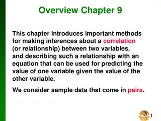
Overview Chapter 9 This chapter introduces important methods for making inferences about a correlation (or relationship) between two variables, and describing such a relationship with an equation that can be used for predicting the value of one variable given the value of the other variable. We consider sample data that come in pairs.
Key Concept Section 9.1 This section introduces the linear correlation coefficient r, which is a numerical measure of the strength of the relationship between two variables representing quantitative data. Because technology can be used to find the value of r, it is important to focus on the concepts in this section, without becoming overly involved with tedious arithmetic calculations.
A correlation is a relationship between two variables. The data can be represented by the ordered pair (x, y) where x is the independent variable and y is the dependent variable. Definition
Definition The linear correlation coefficientr measures the strength of the linear relationship between paired x- and y- quantitative values in a sample.
Exploring the Data We can often see a relationship between two variables by constructing a scatterplot. The following shows scatterplots with different characteristics.
1. The sample of paired (x, y) data is a random sample of independent quantitative data. 2. Visual examination of the scatterplot must confirm that the points approximate a straight-line pattern. 3. The outliers must be removed if they are known to be errors. The effects of any other outliers should be considered by calculating r with and without the outliers included. Requirements
n represents the number of pairs of data present. denotes the addition of the items indicated. x denotes the sum of all x-values. x2 indicates that each x-value should be squared and then those squares added. (x)2 indicates that the x-values should be added and the total then squared. xy indicates that each x-value should be first multiplied by its corresponding y-value. After obtaining all such products, find their sum. r represents linear correlation coefficient for a sample. represents linear correlation coefficient for a population. Notation for the Linear Correlation Coefficient
nxy–(x)(y) r= n(x2)– (x)2n(y2)– (y)2 Formula The linear correlation coefficientr measures the strength of a linear relationship between the paired values in a sample. But…it’s easy because Calculators can compute r Go to STAT, Calc, LinReg(ax+b) L1,L2 to find r
Interpreting r Using Table 11 in Appendix B (p. A28): If the absolute value of the computed value of r exceeds the critical value in Table 11, conclude that there is a linear correlation. Otherwise, there is not sufficient evidence to support the conclusion of a linear correlation.
Round to three decimal places so that it can be compared to critical values in Table 11. Use calculator or computer if possible. Rounding the Linear Correlation Coefficient r
Data x 3 5 1 8 3 6 5 4 y Example: Calculating r Using the simple random sample of data below, find the value of r.
Data x 3 5 1 8 3 6 5 4 y nxy–(x)(y) r= n(x2)– (x)2n(y2)– (y)2 4(61)–(12)(23) r= 4(44)– (12)24(141)– (23)2 -32 r= = -0.956 33.466 Example: Calculating r - cont
Example: Calculating r - cont Given r = - 0.956, if we use a 0.05 significance level we conclude that there is a linear correlation between x and y since the absolute value of r exceeds the critical value of 0.950. However, if we use a 0.01 significance level, we do not conclude that there is a linear correlation because the absolute value of r does not exceed the critical value of 0.999.
Example: Old Faithful Given the sample data in the previous table, find the value of the linear correlation coefficient r, then refer to Table 11 to determine whether there is a significant linear correlation between the duration and interval of the eruption times. Using the same procedure previously illustrated, we find that r = 0.926. Referring to Table 11, we locate the row for which n = 8. Using the critical value for = 0.05, we have 0.707. Because r = 0.926, its absolute value exceeds 0.707, so we conclude that there is a linear correlation between the duration and interval after the eruption times.
1. –1 r 1 2. The value of r does not change if all values of either variable are converted to a different scale. 3. The value of r is not affected by the choice of x and y. Interchange all x- and y-valuesand the value of r will not change. 4. r measures strength of a linear relationship. Properties of the Linear Correlation Coefficient r
Interpreting r : Explained Variation The value of r2(the coefficient of determination) is the proportion of the variation in y that is explained by the linear relationship between x and y.
Example: Old Faithful Using the duration/interval data in Table 10-1, we have found that the value of the linear correlation coefficient r = 0.926. What proportion of the variation of the interval after eruption times can be explained by the variation in the duration times? With r = 0.926, we get r2 = 0.857. We conclude that 0.857 (or about 86%) of the variation in interval after eruption times can be explained by the linear relationship between the duration times and the interval after eruption times. This implies that 14% of the variation in interval after eruption times cannot be explained by the duration times.
1. Causation: It is wrong to conclude that correlation implies causality. 2. Linearity: There may be some relationship between x and y even when there is no linear correlation. 3. Coincidence: Although it may be possible to find a correlation – sometimes it is merely coincidence. Common Errors Involving Correlation