Random Number Generators for Cryptographic Applications (Part 2)
700 likes | 915 Vues
Random Number Generators for Cryptographic Applications (Part 2). Werner Schindler. Federal Office for Information Security (BSI), Bonn. Bonn, January 24, 2008. Outline (Part 2). Repetition of crucial facts Design and evaluation criteria for physical RNGs general advice stochastic model

Random Number Generators for Cryptographic Applications (Part 2)
E N D
Presentation Transcript
Random Number Generators for Cryptographic Applications (Part 2) Werner Schindler Federal Office for Information Security (BSI), Bonn Bonn, January 24, 2008
Outline (Part 2) • Repetition of crucial facts • Design and evaluation criteria for physical RNGs • general advice • stochastic model • entropy • online tests, tot test, self test • AIS 31 and ISO 18031 • Conclusion
deterministic non-deterministic (true) pure hybrid physical non-physical pure hybrid pure hybrid Classification RNG
General Requirements (I) R1: Random numbers should not show statistical weaknesses (i,e., they should pass statistical “standard tests”). R2: The knowledge of subsequences of random numbers shall not allow to practically compute predecessors or successors or to guess them with non-negligibly larger probability than without knowledge of these subsequences.
General Requirements (II) R3: It shall not be practically feasible to compute preceding random numbers from the internal state or to guess them with non-negligibly larger probability than without knowledge of the internal state. R4: It shall not be practically feasible to compute future random numbers from the internal state or to guess them with non-negligible larger probability than without knowledge of the internal state.
Ideal RNGs • Even with maximum knowhow, most powerful technical equipment and unlimited computational power an attacker has no better strategy than “blind guessing” (brute force attack). • Guessing n random bits costs 2n-1 trials in average. • The guess work remains invariant in the course of the time. • An ideal RNG clearly meets Requirements R1 - R4 • An ideal RNG is a mathematical construct.
external interface digital algorithmic postprocessing buffer (optional) (optional; with or without memory) digitised analog signal (das-random numbers) internal r.n. external r.n. PTRNG (schematic design) analog noise source
Noise source • The noise source is given by dedicated hardware. • The noise source exploits, for example, • noisy diodes • free-running oscillators • radioactive decay • quantum photon effects • ... Physical RNGs (should) aim at information theoretical security.
Development and Security Evaluation of PTRNGs The challenge is threefold: • Development and implementation of a strong RNG design • Verification that design and implementation are indeed strong • effective detection mechanisms for possible non-tolerable weaknesses of random numbers while the PTRNG is in operation
The central part of a PTRNG security evaluation is to verify Requirement R2. • R1 is easy to fulfil and to check. Apart from very unusual designs R3 and R4 are “automatically” fulfilled.
Optimal guessing strategy • Let X denote a random variable that assumes values in a finite set S = {s1, ... ,st}. • The optimal guessing strategy begin with those values that are assumed with the largest probability.
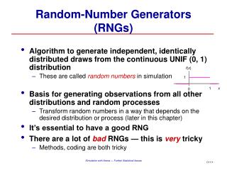
Guess work and entropy (I) • Goal of a PTRNG security evaluation: Try to estimate the expected number of guesses that is necessary to find a random number with a certain (reasonable) probability. • For real-world PTRNGs it is usually yet not feasible to determine this value directly. • Instead, entropy shall provide a reliable estimator. • Goal: Determine (at least) a lower bound for the entropy per bit (general purpose RNG).
Evaluation Note:Entropy is a property of random variables and not of values that are assumed by these random variables (here: random numbers). • In particular, entropy cannot be measured as temperature, voltage etc. • General entropy estimators for random numbers do not exist.
Warning Warning Warning • The test values of Maurer‘s „universal entropy test“ and of Coron‘s refinement are closely related to the entropy per random bit if the respective randomvariables fulfil several conditions. • If these conditions are not fulfilled (e.g. for pure DRNGs!) the test value need not be related to the entropy. • The adjective “universal” has caused a lot of confusion in the past.
Fundamental model assumptions • We interpret random numbers as realizations of random variables. • Although entropy is a property of random variables in the following we loosely speak of the “(average) entropy per random number” instead of “(average) gain of entropy per corresponding random variable”. • A reliable security evaluation of a PTRNG should be based on a stochastic model.
Guess work and entropy (II) • The min entropy is the most conservative entropy measure. For arbitrary distribution of X a lower bound for the guesswork can be expressed in terms of the min entropy while the Shannon entropy may pretend larger guess work.
x1,...,xnS Conditional entropy (I) Let X1,X2,... denote random variables that assume values in a finite set S = {s1, ... ,st}. The conditional entropy H(Xn+1 | X1,...,Xn) = H(Xn+1 | X1=x1,...,Xn=xn) *Prob(X1 = x1,…,Xn = xn) quantifies the increase of the overall entropy when augmenting Xn+1 to the sequence X1,...,Xn.
Conditional entropy (II) H(X1,...,Xn, Xn+1) = H(X1,...,Xn) H(Xn+1 | X1,...,Xn) = ... = H(X1) H(X2 | X1) ... H(Xn+1 | X1,...,Xn) This formula is very useful to determine the entropy of dependent sequences. There is no pendant for the min entropy.
Guess work and entropy (III) • Assume that X1,X2,... denotes a sequence of binary-valued iid (identically and identically distributed) random variables. Unless n is too small H(X1,X2,...,Xn)/n log2(E(number of guesses per bit)) • The assumption “iid” may be relaxed, e.g. to “stationary with finite memory”. • If the random variables X1,X2,...,Xn are ‘close’ to the uniform distribution all parameters give similar Renyi entropy values.
Guess work and entropy (IV) • (At least) the internal random numbers usually fulfil both the second and the third condition. • Hence we use the Shannon entropy in the following since it is easier to handle than the min entropy ( conditional entropy).
The stochastic model (I) • Goal: Estimate the increase of entropy per internal random number • Ideally, a stochastic model should specify a family of probability distributions that contains the true distribution of the internal random numbers. • It should at least specify a family of distributions that contain the distribution of the • das random numbers or • of ‚auxiliary‘ random variables that allow to estimate the increase of entropy per internal random number.
Example 5: Coin Tossing • PTRNG: A single coin is tossed repeatedly. "Head" (H) is interpreted as 1, "tail" (T) as 0. • Stochastic model: • The observed sequence of random numbers (here: heads and tails) are interpreted as values that are assumed by random variables X1,X2,… . • The random variables X1,X2, … are assumed to be independent and identically distributed. (Justification: Coins have no memory.) • p : = Prob(Xj = H) [0,1] with unknown parameter p
Example 5: Coin Tossing (II) • Note: A physical model of this experiment considered the impact of the mass distribution of the coin on the trajectories. The formulation and verification of the physical model is much more complicated than for the stochastic model.
The stochastic model (II) • A stochastic model is not equivalent to a physical model. In particular, it does not provide the exact distribution of the das random numbers or the internal numbers in dependency of the characteristics of the components of the analog part. • Instead, the stochastic model only specifies a class of probability distributions which shall contain the true distribution (see also Example 5). • The class of probability distributions usually depends on one or several parameters.
The stochastic model (III) • The stochastic model shall be verified by measurements / experiments. • The parameter(s) of the true distribution are guessed on basis of measurements. • The stochastic model allows the design of effective online tests that are tailored to the specific RNG design.
Entropy estimation (based on the stochastic model): • Observe a sample x1,x2, …, xN. Set p := #j N | xj = H / N • To obtain an estimator H(X1) for H(X1) substitute p into the entropy formula: H(X1) = - ( p* log2 (p) + (1-p) * log2(1-p)) ~ ~ ~ ~ ~ ~ ~ ~ Example 5: Coin Tossing (III)
The stochastic model (IV) • For PTRNGs the justification of the stochastic model is usually more complicated and requires more sophisticated arguments. • To estimate entropy the parameter(s) are estimated first, and therefrom an entropy estimate is computed (cf. Example 5). • If the random numbers are not independent the conditional entropy per random bit has to be considered.
43 bit LFSR ring oscillator 1 k bit permutation output (internal random number) permutation k bit 37 bit CASR ring oscillator 2 Example 6 (I) PTRNG design proposed in [Tk] CASR = Cellular Automaton Shift Register (GF(2)-linear)
Example 6 (II) Two free-running ring oscillators clock the LFSR and the CASR, respectively. The intermediate time between two outputs of random numbers shall exceed a minimum number of LFSR and CASR cycles. • noise source: ring oscillators • das random numbers: number of cycles of the LFSR and CASR between subsequent calls of the RNG • internal state: current states of the LFSR and CASR • internal random number: k-bit output string
Example 6 (III): Dichtl’s attack • Original parameters: k =32 • Assume that the attacker knows • the three following 32-bit random numbers • the number of intermediate cycles of the LFSR and CASR. • all implementation details (permutation etc.) • Notation: state of the LFSR at time t=0: (a1,...,a43) state of the CASR at time t=0: (a´1,...,a´37) • This gives an (over-determined!) system of 96 GF(2)-linear equations in 80 variables with solution (a1,...,a43,a´1,...,a´37).
Example 6 (IV) • Original parameters: k = 32; minimum waiting time between two outputs: 86 LFSR cycles, 74 CASR cycles Goal: Determine the conditional entropy H(Yn+1| Y1, ...,Yn) (internal random numbers) in dependency of k and the time between two outputs of random numbers.
Example 6 (V) Upper entropy bound: At least in average, H(Yn+1| Y1, ...,Yn) H(V1,n+1) + H(V2,n+1) where the random variables V1,n+1 and V2,n+1 describe the number of cycles of the two ring oscillators between two calls of the RNG Lower entropy bound: Estimate the entropy from below that the output function extracts from the internal state.
Example 6 (VI) • In [Sch3] a thorough analysis of the PTRNG design is given. Both a lower and an upper entropy bound per internal random bit are given that depend on • the intermediate time between subsequent outputs in multiples of the average cycle time • the jitter of the ring oscillators • the bit length k of the internal random numbers.
Example 6 (VII): Numerical values • = average cycle length • = 0.01 (optimistic assumption) Time k internal state entropy per random number (increase of entropy) 10000 1 4,209 0.943 10000 2 4.209 0.914 10000 3 4.209 0.866 60000 1 6.698 0.991
Example 7 internal random numbers
time 0 s 2s 3s 4s 5s sw(1)=5 sw(2)=5 sw(3)=7 sw(4)=6 sw(5)=8 | = clock signal | = (0-1)-comparator switch swn= # (0-1) crossings in time interval ((n-1)s,ns] das random number: rn = swn internal random number: yn+1 = yn + rn+1 (mod 2)
Strategy • Goal: Determine (at least a lower bound for) H(Yn+1 | Y0, ...,Yn) • Remark: Example 7 contains joint research work with Wolfgang Killmann.
Notation • t1,t2,....: time periods between subsequent switches of the comparator • zn: smallest index m for which t0+t1+t2+...+tm>sn • wn = t0+t1+t2+...+tm -sn (or, equivalently, wn t0+t1+t2+...+tm (mod s) )wn denotes the time between sn and the next comparator switch
Stochastic model (II) • It is reasonable to assume that the noise source is in equilibrium state shortly after start-up. • The stochastic process T1,T2,... is assumed to be stationary (not necessarily independent !).
Stochastic Model (III) The das random numbers in Example 6 and Example 7 (and the das random numbers of other RNGs designs) can be modelled as follows: T1,T2,… are stationary Rn := Zn- Zn-1 with Zn := min {m N | T0 + … + Tm >sn}
General remark • Even if two different RNG designs fit to this model • the distribution of the random variables T1,T2,… and thus of R1,R2,... may be very different.
Stationarity • The stochastic process T1,T2,... is assumed to be stationary • Under weak assumptions (essentially, the partial sums T1+T2 +... + Tm (mod s) should tend to the uniform distribution on [0,s))it can be shown that the sequences W1,W2,... and R1,R2,... are stationary, too. • Strategy: Study the stochastic process R1, R2,... first.
Stochastic model (IV) • Definition • V(u) := # 0-1 switchings in [0,u] • μ = E(Tj) • σ² := generalized variance of T1,T2,... • ( . ):= cumulative distribution function of the standard normal distribution
Auxiliary variables Lemma: For u = v ∙ μ
Entropy (II) Under mild regularity assumptions on the random variables Tj the term with moderate a>0 should provide a conservative estimate for H(Rn+1 | R0,...Rn). The size of a depends on the distribution of the random variables Tj .
GW(du) E ( E ( V ) +1|W0=u) R +...+ R = - ( ) js u 1 j js k ò GW(du) E ( V +1) - ( ) js u 0 Autocovariance Theorem 1 : Let GW(.) denote the cumulative distribution function of Wn . Then js k k ò (i) 0 (ii) For k = 2, j=1,2, ... this provides the auto-correlation function of the stationary process R1,R2,... (iii) If the Tj are iid the above formula is exact. If these Tj have continuous cumulative distribution function F(.) then GW(u) = (1-F(u)) /.
Entropy (III) Theorem 2 (special case): Assume that the random variables T1,T2, ... are iid with continuous cumulative distribution function F(∙). Then s - 1 F ( u) ò H ( R | R ,..., R ) H ( V du ) + - 1 0 ( ) n n s u 0
Example 7 (II) • Experimental results: 105 random bits per second with entropy per bit > 1-10-5. • Numerical values: Erlang (2,)-distribution • a) s = 6*E(T1): Var(R1)=3.4 , corr(R1,R2)=-0.06, corr(R1,R3)=-0.004, ... • b) s = 9*E(T1): Var(R1)= 4.95, corr(R1,R2)= -0.046, corr(R1,R3)= -0.00005, ...
PTRNGs in operation: Potential risks • Worst case: total breakdown of the noise source • Ageing effects, tolerances of components of the noise source and external influences might cause the generation of random numbers with unacceptably low quality. Such events must be detected certainly so that appropriate responses can be initiated.