VII. Observation-Parameter Statistics
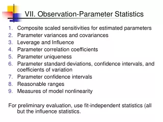
VII. Observation-Parameter Statistics. Composite scaled sensitivities for estimated parameters Parameter variances and covariances Leverage and Influence Parameter correlation coefficients Parameter uniqueness Parameter standard deviations, confidence intervals, and coefficients of variation

VII. Observation-Parameter Statistics
E N D
Presentation Transcript
VII. Observation-Parameter Statistics • Composite scaled sensitivities for estimated parameters • Parameter variances and covariances • Leverage and Influence • Parameter correlation coefficients • Parameter uniqueness • Parameter standard deviations, confidence intervals, and coefficients of variation • Parameter confidence intervals • Reasonable ranges • Measures of model nonlinearity For preliminary evaluation, use fit-independent statistics (all but the influence statistics.
1. Composite Scaled Sensitivities (Book, p. 124-125) • CSS were used initially to help decide which parameters to estimate. • Recall that they indicate the total amount of information provided by the observations for the estimation of each individual parameter. • Can be also be used as an initial gauge of the reliability with which the parameters are estimated. Parameters with larger values of CSS are generally estimated more reliably than those with smaller values of CSS. • After the regression has converged, it is important to recalculate CSS for all parameters, to check whether the conclusions made for the initial CSS about which parameters to estimate still apply. Should additional parameters be estimated? Should changes be made in the use of prior information? • DO EXERCISE 7.1a (p. 145) • What is the difference between initial and final CSS values? • Effect of model nonlinearity and scaling? • Use CSS to explain small weighted residuals for prior information.
1. Composite Scaled Sensitivities Composite scaled sensitivities from the starting steady-state model • An alternative: • The relative parameter coefficients of variation can also be plotted. • - They equal the parameter standard deviation divided by the parameter value. • Not fit-independent, but all are multiplied by the same value of the standard error of the regression so relative values are useful. • Account for parameter correlation Composite scaled sensitivities from the final steady-state model (Book, Fig. 7-5a, p. 146)
2. Parameter Variances and Covariances The variance-covariance matrix for the parameters is:. (Hill and Tiedeman, 2007, p. 125, eq 7.1) V(b)=s2(XTwX) -1 b is a vector of parameter values s2 is he calculated error variance (measure of model fit) X is the matrix of sensitivities of the simulated equivalents to the observations, calculated at b w is the weight matrix
2. Parameter variance-covariance matrix • V(b)=s2(XTwX)-1 • Five versions • With optimized parameter values and only optimized parameters. • With optimized parameter values and all defined parameters • With nonoptimal parameter values • Alternate observation sets – observations omitted or added • With predictions • For versions a and b, s2 is calculated using optimal parameter values and statistics affected by s2 can be meaningful • For versions c, d, and e, use statistics for which s2 divides out • For now we will work with version (a)
2. Parameter Variances and Covariances(book p. 126) • The diagonal elements of the matrix are the parameter variances; the off-diagonal elements are the parameter covariances. For a 3 parameter problem, the matrix is: Var (1) Cov(1,2) Cov(1,3) Cov (2,1) Var (2) Cov (2,3) Cov (3,1) Cov (3,2) Var (3)
2. Parameter Variances and Covariances (Book, p. 126) • The parameter variance-covariance matrix is used to evaluate parameter uncertainty and parameter correlation. • Generally, we use statistics computed from the parameter variance-covariance matrix, rather than elements of the matrix itself.
2. Regression Parameter Variances and Covariances • In regression, the parameter values are estimated indirectly using observations. • This can be accomplished because the simulation model is based on equations that relate observations to parameter values. • Because of this indirect way of estimating parameter values, parameter variances and covariances are calculated using sensitivities. • Interpretation of the variance and correlation of parameters estimated by regression : • The variance indicates the range over which a parameter value could extend without affecting model fit too adversely. • The parameter correlation coefficients indicate whether coordinated changes in the parameter values could produce the same simulated values and, therefore, the same model fit.
~Var(b2) ~Var(b1) 2. Parameter Variances and Covariances b2 Linear objective function: No correlation, b1 less sensitive minimum Can change b1 and have little change in the objective function. Objective function changes more quickly with b2 b1
2. Parameter Variances and Covariances b2 Linear objective function Strong, negative correlation Can change b1 and b2 together and have little change in the objective function minimum b1
3. Leverage and Influence • Based on V(b) • Important to understand the role that observations play in the regression • Estimates can be largely affected by very few observations • Two characteristics are important • Leverage – depends only on the type, location, and time of the observation • Influence – depends on the observed value as well
( ) - 1 = w T T h x X X x i i i where h is leverage of ith parameter i x is a vector composed of the scaled sensitivities of the ith i parameter or the transpose of the ith row of the X matrix 3. Leverage (p. 134) • Leverage Statistics identify observations for which observed values potentially have a big effect on regression results • If the observation is inconsistent with other observations, the observation will dominate the estimated parameter values if it has high leverage. • Measures a potential effect. • May or may not be an actual effect.
3. Leverage for linear regression • Leverage = (1/n) + [(xi-(Sx/n))2]/SSx • Leverage is large when the X for an observation is far from the mean of the X’s. • In linear regression, the X values are equivalent to our sensitivities. • The idea that high leverage parameters are those for which the sensitivities are somehow different carries over to multiple, nonlinear regression.
3. Influence: Cook’s D and DFBETAS • Influence Statistics incorporate calculated residuals to determine the actual effect of the observation in the regression • Cook’s D is a measure of how a set of parameter estimates would change with omission of an observation, relative to how well the parameters are estimated given the entire set of observations (in file with extension ._rc) • DFBETAS measures the importance of one observation to one parameter. Specifically, the influence of observation i on parameter j, scaled by the variance of parameter j when estimated using all observations (in file with ._rb) • residual_analysis.exe calculates these measures and prints them in UCODE_2005 data-exchange files
3. Leverage vs. Influence High leverage Low influence 19 Exclude obs 18 All obs High leverage High influence Exclude obs 19 18 Regression line when the more influential of the points considered is omitted from the regression
Exercises • EXERCISE 7.1b: Evaluate leverage statistics (p. 146) • Statistics needed are in ex5.2c_ucode._so • EXERCISE 7.1c: Evaluate importance of using influence statistics (p. 146) • DFBETAS are in file ex5.2c_ucode._rb • Cook’s D are in file ex5.2c_ucode._rc • Produced in exercise 6.2e by running the residual_analysis computer program • Use the equations in Hill and Tiedeman (2007) to calculate the critical values. Compare them to the graphs to identify influential observations. • Cood • Cook’s D: 4/(ND+NPR) DFBETAS: 2/(ND+NPR)1/2
4. Parameter Correlation Coefficients (Book, p. 127) • Parameter correlation coefficients (from the _pcc file) are used primarily to assess parameter uniqueness • Computed fromparameter variance-covariance matrix values • Correlation coefficients are typically presented as a matrix. • Independent of model fit (s2 cancels out in calculation). Correlation coefficients depend only on sensitivities of the simulated equivalents to the parameters, and weights. • Because of model nonlinearity, parameter correlation coefficients are a function of parameter values. • Variances are always positive, covariances (and therefore, correlation coefficients) can be positive or negative.
4. Parameter Correlation Coefficients • If the absolute value of a correlation for a parameter pair is greater than about 0.95, then it may not be possible to estimate the 2 parameters uniquely using the available regression data. Changing the parameter values in a coordinated manner may produce very similar model results. • In this case, it is essential to restart the regression with different initial parameter values and check whether the regression converges to the same estimates. If not, then the parameter estimates are not unique • Absolute values close to 1.0 may also cause failure of the regression to converge to a set of ‘optimal’ values. • DO EXERCISE 7.1d (p. 148)
4. Correlation Coefficients and Inaccurate Sensitivities • If using a perturbation method to calculate sensitivities using, for example, UCODE_2005 or PEST, the sensitivities generally are less accurate than those computed using the sensitivity equation method using, for example, MODFLOW-2000. • Inaccurate sensitivities produce parameter correlation coefficients close to 1.0 that are reliable, but correlation coefficients far from 1.0 that may be inaccurate. The problem becomes worse as one or both of the parameters involved in the correlation become less sensitive. • Correlation coefficients far from 1.0 may mean either there is a lack of correlation or the correlations are not accurate enough. • It is important to test for nonuniqueness even if the calculated correlations are not close to 1.0 • FINISH EXERCISE 7.1d
4. Parameter Correlation Coefficients • EXERCISE 7.2: Consider all the different correlation coefficients presented (p. 155) R = (6.11a) = (6.18) (7.5)
5. Further tests for nonunique parameters • While useful, for a variety for reasons parameter correlation coefficients can fail to detect nonunique solutions. • Furthe investigation methods include starting the regression from alternative starting values of the parameters and using global sensitivity analysis and regression methods. • In this class we consider alternative starting values of the parameters.
Exercise 7.1e. Detecting non-unique parameter estimates – instructions for MFI2005 First, perform a regression run without flow observation and prior information: • In MFI2K, save the ex5.2c dataset as dataset ex7.1e and use the ex7.1e dataset in this exercise • To omit the flow observation, click on “Deactivate” under the Options menu in MFI, and deactivate RVOB • In “Observations>Single-Head Observations”, make the name of the output file ex7.1e._os • From the UCODE menu, remove the prior information equations • Perform regression • Do part 1 of the Problem on p. 150 of Hill and Tiedeman • Run UCODE_2005 with SensitivityAnalysis=yes to obtain a parameter correlation matrix Next, include the flow observation and prior information, and start the regression from different initial values: • Include the flow observation by activating RVOB • In the PES file, include the prior information equations, and change MAX-ITER to 10 • In the SEN file, change the starting parameter values to the values in set 1 of table 10, perform nonlinear regression, and rename the _ot file from this run. Then, change the values to those in set 2 of table 10, and perform nonlinear regression • Do part 2 of the Problem on p. 151 of Hill and Tiedeman
6. Parameter Standard Deviation andCoefficient of Variation (Book, p. 127) • The parameter standard deviation (σ) for parameter bj is the square root of the parameter variance (on the diagonal of the parameter variance-covariance matrix): • The parameter standard deviation is easier to interpret than the parameter variance, because it is in the same units as the parameter value. • The parameter coefficient of variation is: • The coefficient of variation is dimensionless, and can be used to compare the relative precision of different parameter estimates
7. Individual Linear Confidence Intervals (Book, p. 138) • The linear individual confidence interval (CI) on a parameter is calculated as: • A 95 percent individual linear CI on a parameter has a 95 percent probability of containing the true parameter value(when the model is sufficiently linear with respect to the parameters)
7. Individual Linear Confidence Intervals • Student-t probability distribution: Similar to normal distribution except adjusts for smaller sample sizes. As n becomes large, the distribution approaches the normal distribution • Width of a confidence interval can be thought of as precision of estimate • Three important assumptions are made in deriving the linear confidence intervals: • The model is correct • The parameter values are normally distributed • The model is linear near the optimal values
7. Individual Linear Confidence Intervals • For a linear model, the parameter estimates are normally distributed if the true observation errors are normally distributed. • However, because the true errors are unknown, we analyze the weighted residuals instead, by constructing a normal probability plot and evaluating RN2. • Model linearity can be evaluated using the modified Beale’s measure (exercise 7.3) • DO EXERCISE 7.1f (p. 151): Evaluate precision by examining standard deviations, linear confidence intervals, and coefficients of variation
7. Linear 95% Confidence Intervals on Estimated Parameter Values If the model and weighting are correct and the mean of the true errors is zero, there is a 95% chance that the true parameter values vall within the calculated ranges. Fig. 7.7, p. 153
Range of Reasonable Values Parameter Value 1 2 3 Situation 8. Comparing Estimated Parameter Values with Reasonable Ranges (Book, p. 140) • It is important to compare the regression estimates of the parameter and the calculated confidence intervals with the reasonable ranges of parameter values. (But you set the reasonable ranges, so be careful.) • 3 common situations: 1: Parameter estimate and most of confidence intervals lie within reasonable range 2: Parameter estimate and confidence intervals lie outside reasonable range 3: Parameter estimate lies outside the range but part of confidence intervals lies within the range
Range of Reasonable Values Parameter Value 1 2 3 8. Comparing Estimated Parameter Values with Reasonable Ranges • Situation 1: Desirable – enough information to estimate the parameter precisely, and the estimate is consistent with independent information (we have learned something: the probable range is smaller than the original range of reasonable values) • Situation 2: Problematic – enough information to estimate the parameter precisely, but the estimate is inconsistent with independent information (we need to reconsider model, choice of parameters, measurements …: why does the outcome go against our expectations) • Situation 3: Inconclusive - there is enough information to estimate the parameter, but not with much precision (we did not learn anything new)
Range of Reasonable Values Parameter Value 1 2 3 Situation 8. Comparing Estimated Parameter Values with Reasonable Ranges • Situation 3: Modeler needs to think about (1) what additional data could provide more information towards estimating the parameter, and (2) improvements to the conceptual model of the system. • Consider adding more observation data, such as flows or concentrations • Regression estimate of parameter may become more reasonable and CI may become smaller • Situations 2 and 3: Adding prior does not address the fundamental problem. There is enough information for the regression to converge to a particular parameter value. The modeler needs to think about what is causing the unreasonable estimates. • DO EXERCISE 7.1g (p. 153) Compare estimated values with reasonable ranges
Confidence intervals, starting, final, and true values, compared to reasonable ranges (Book, Figure 7-7, p.153) GW_Chart can make graphs like these. _pc
9. Test linearity of model • Linear confidence intervals are only valid when the model is sufficiently linear. • Model linearity is evaluated by using the modified Beale’s measure and total and intrinsic model linearity measures
Modified Beale’s Measure. ex7.3_ucode.#modlin USING FSTAT = 3.8660 , BEALES MEASURE = 35.435 IF BEALES MEASURE IS GREATER THAN 0.26 , THE MODEL IS NONLINEAR. IF BEALES MEASURE IS LESS THAN 0.23E-01, THE MODEL IS EFFECTIVELY LINEAR, AND LINEAR CONFIDENCE INTERVALS ARE FAIRLY ACCURATE IF THE RESIDUALS ARE NORMALLY DISTRIBUTED.
From output file ex7.3_ucode.#modlinadv_conf ########################################################## ########### ########### TOTAL NONLINEARITY (BNT).......... = 45.433 ########### INTRINSIC NONLINEARITY (BNI)...... = 0.12908 ########### ###########CRITICAL VALUES FOR BOTH MEASURES: ########### >1.0 highly nonlinear ########### 0.09 to 1.0 non-linear ########### 0.01 to 0.09 moderately nonlinear ########### <0.01 effectively linear ##########################################################
End of VII. Parameter Statistics • Composite scaled sensitivities for estimated parameters • Parameter variances and covariances • Leverage and Influence • Parameter correlation coefficients • Parameter uniqueness • Parameter standard deviations, confidence intervals, and coefficients of variation • Parameter confidence intervals • Reasonable ranges • Measures of model nonlinearity

