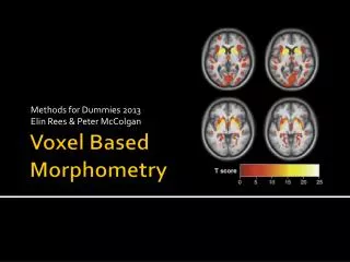
Voxel Based Morphometry

1. Methods for Dummies 2013 Elin Rees & Peter McColgan Voxel Based Morphometry

2. Contents • Longitudinal fluids • Interpretation • Issues • Multiple comparisons • Controlling for TIV • Global or local change • Interpreting results • Summary • General idea • Pre-Processing • Spatial normalisation • Segmentation • Modulation • Smoothing • Statistical analysis • GLM • Group comparisons • Correlations

3. General Idea • Uses Statistical Parametric Mapping software • ‘Unbiased’ technique • Pre-processing to align all images • Parametric statistics at each point within the image • Mass-univariate • Statistical parametric map showing e.g. • differences between groups • regions where there is a significant correlation with a clinical measure

4. Pre-Processing: Unified Segmentation = iterative tissue classification + normalisation + bias correction • Segmentation: • Models the intensity distributions by a mixture of Gaussians, but using tissue probability map (TPM) to weight the classification • TPM = priors of where to expect certain tissue types • Affine registration of scan to TPM • Normalisation: • The transform used to align the image to the TPM used to normalise the scan to standard (TPM) space • parameters calculated but not applied • Corrects for global brain shape differences • Bias correction: • Spatially smoothesthe intensity variability, which is worse at higher field strengths

5. DARTEL • Registration of GM segmentations to a standard space 1) Applies affine parameters into TPM space 2) Additional non-linear warp to study specific space • Study-specific grey matter template • Constructs a flow field so one image can slowly ‘flow’ into another • Allows for more precise inter-subject alignment • Involves prior knowledge e.g. stretches, scales, shifts and warps = DiffeomorphicAnatomical Registration using ExponentiatedLie algebra registration

6. Pre-Processing: Modulation • Spatial normalisation removes differences between scans • Modulation of segmentations puts this information back • Rescaling the intensities dependent on the amount of expansion/contraction - if not much change needed, not much intensity change E.g. Native = 1 1 Unmodulated warped = 1 1 1 1 Modulated = 2/3 1/3 1/3 2/3 = lower in the middle where imaged stretched but total is preserved.

7. Pre-Processing: Smoothing • Gets rid of roughness and noise to produce data in a more normal distribution • Removes some registration errors • Kernel defined in terms of FWHM (full width at half maximum) of filter • 7-14mm kernel • Analysis is most sensitive to effects that match the shape and size of the kernel • Match Filter Theorem • Kernel takes weighted average of the surrounding intensities • Smaller kernels mean results can be localised to a more precise region • Less smoothing needed if DARTEL used • In an ideal world this would not be needed

8. Results • Voxel-wise (mass-univariate) independent statistical tests for every single voxel • Group comparison: • Regions of difference between groups • Correlation: • Region of association with test score

9. Statistical Analysis • Test group differences in e.g. grey matter BUT • which covariates e.g. age, gender etc.? • which search volume? • what threshold? • correction for multiple comparisons? • Ridgeway et al. 2008: Ten simple rules for reporting voxel-based morphometrystudies • Multiple methodological options available • Decisions must be clearly described • Henley et al. 2009: Pitfalls in the Use of Voxel-Based Morphometry as a Biomarker: Examples from Huntington Disease

10. Statistical Analysis • GLM Y = Xβ + ε • Intensity for each voxel (V) is a function that models the different things that account for differences between scans: V = β1(Subject A) + β2(Subject B) + β3(covariates) + β4(global volume) + μ + ε V = β1(test score) + β2(age) + β3(gender) + β4(global volume) + μ + ε

11. Statistical Analysis • SPM • Mass univariate independent statistical tests for every voxel ~ 1000,000 • Regions of significantly less grey matter intensity between subjects and controls • Regions showing a significant correlation with test score or clinical measure

12. Statistical Analysis • Multiple Comparisons • Introducing false positives when dealing with one than one statistical comparison • One t-test with p < .05 • a 5% chance of (at least) one false positive • 3 t-tests, all at p < .05 • All have 5% chance of a false positive • So actually you have 3 x 5% chance of a false positive =15% chance of introducing a false positive

13. Statistical Analysis • How big is the problem? • In VBM, depending on your resolution • 1000000 voxels • 1000000 statistical tests • do the maths at p < .05! • 50000 false positives • So what to do? • Bonferroni Correction • Random Field Theory/ Family-wise error • False Discovery Rate • Small Volume Correction

14. Statistical Analysis • Bonferroni-Correction (controls false positives at individual voxel level): • divide desired p value by number of comparisons • .05/1000000 = p < 0.00000005 at every single voxel • Not a brilliant solution (false negatives) • Added problem of spatial correlation data from one voxel will tend to be similar to data from nearby voxels

15. Statistical Analysis • Family Wise Error (FWE) • Probability that one or more of the significance tests results is a false positive within the volume of interest • SPM uses Gaussian Random Field Theory (GRFT) • GRFT finds right threshold for a smooth • statistical map which gives the required • FWE. It controls the number of false • positive regions rather than voxels • Allows multiple non-independent tests

16. Statistical Analysis • False Discovery Rate • Controls the expected proportion of false positives among suprathreshold voxels only • Using FDR, q<0.05: we expect 5% of the voxels for each SPM to be false positives (1,000 voxels) • Bad: less stringent than FWE so more false positives • Good: fewer false negatives (i.e. more true positives) • More lenient may be better for smaller studies

17. Statistical Analysis • Small Volume Correction • Hypothesis driven and ideally based on previous work • Place regions of interest over particular structures • Reduces the number of comparisons • Increases the chance of identifying significant voxels in a ROI

18. Other Issues in VBM • Controlling for total intracranial volume (TIV) brain A brain B Differences without accounting for TIV brain A brain B differences after TIV has been “covaried out” (Differences uniformallydistributed with hardly any impact at local level) Uniformly bigger brains may have uniformly more GM/ WM

19. Other Issues in VBM • Global or local change • With TIV: greater volume in A relative to B only in the thin area on the right-hand side • Without TIV: greater volume in B relative to A except in the thin area on the right-hand side Including total GM or WM volume as a covariate adjusts for global atrophy and looks for regionally-specific changes

20. Other Issues in VBM • Interpretation

21. contracting expanding Other Issues in VBM • Longitudinal Analysis: • Fluid Registration • Baseline and follow-up • image are registered together • non-linearly • Voxels at follow-up are • warped to voxels at baseline • Represented visually as • a voxel compression map • showing regions of contraction • and expansion

22. Limitations • Small volume structures: Hippocampus and Caudate, issues with normalisation and alignment • VBM in degenerative brain disease: • normalisation, segementation and smoothing • of atrophied scans

23. Summary • Disadvantages • Data collection constraints (exactly the same way) • Statistical challenges • Results may be flawed by preprocessing steps • Underlying cause of difference unknown • Interpretation of data- what are these changes when they are not volumetric? • Advantages • Fully automated: quick and not susceptible to human error and inconsistencies • Unbiased and objective • Not based on regions of interests; more exploratory • Picks up on differences/ changes at a global and local scale • Has highlighted structural differences and changes between groups of people as well as over time

24. Questions ?