Voxel -Based Morphometry John Ashburner
Voxel -Based Morphometry John Ashburner. Wellcome Trust Centre for Neuroimaging , 12 Queen Square, London, UK. Overview. Voxel -Based Morphometry Morphometry in general Volumetrics VBM p reprocessing followed by SPM Segmentation Dartel Recap. Measuring differences with MRI.

Voxel -Based Morphometry John Ashburner
E N D
Presentation Transcript
Voxel-Based MorphometryJohn Ashburner Wellcome Trust Centre for Neuroimaging, 12 Queen Square, London, UK.
Overview Voxel-Based Morphometry Morphometry in general Volumetrics VBM preprocessing followed by SPM Segmentation Dartel Recap
Measuring differences with MRI • What are the significant differences between populations of subjects? • What effects do various genes have on the brain? • What changes occur in the brain through development or aging? • A significant amount of the difference (measured with MRI) is anatomical. • You need to discount the larger anatomical differences before giving explanations about brain function.
There are many ways to model differences. Usually, we try to localise regions of difference. Univariate models. Using methods similar to SPM Typically localising volumetric differences Some anatomical differences can not be localised. Need multivariate models. Differences in terms of proportions among measurements. Where would the difference between male and female faces be localised? Need to select the best model of difference to use, before trying to fill in the details.
Deformations Could do a multivariate analysis of these (“Deformation-Based Morphometry”).
Relative Volumes Could do a mass-univariate analysis of these (“Tensor-Based Morphometry”).
Voxel-Based Morphometry • Based on comparing regional volumes of tissue. • Produce a map of statistically significant differences among populations of subjects. • e.g. compare a patient group with a control group. • or identify correlations with age, test-score etc. • The data are pre-processed to sensitise the tests to regional tissue volumes. • Usually grey or white matter. • Suitable for studying focal volumetric differences of grey matter.
Volumetry T1-Weighted MRI Grey Matter
Warped Template Original
“Modulation” – change of variables. Deformation Field Jacobians determinantsEncode relative volumes.
Smoothing Each voxel after smoothing effectively becomes the result of applying a weighted region of interest (ROI). Before convolution Convolved with a circle Convolved with a Gaussian
VBM Pre-processing in SPM8 • Use New Segment for characterising intensity distributions of tissue classes, and writing out “imported” images that DARTEL can use. • Run DARTEL to estimate all the deformations. • DARTEL warping to generate smoothed, “modulated”, warped grey matter. • Statistics.
group 1 group 2 Statistical Parametric Mapping… – parameter estimate standard error statistic image orSPM = voxel by voxelmodelling
“Globals” for VBM • Shape is really a multivariate concept • Dependencies among volumes in different regions • SPM is mass univariate • Combining voxel-wise information with “global” integrated tissue volume provides a compromise • Using either ANCOVA or proportional scaling (ii) is globally thicker, but locally thinner than (i) – either of these effects may be of interest to us.
Total Intracranial Volume (TIV/ICV) • “Global” integrated tissue volume may be correlated with interesting regional effects • Correcting for globals in this case may overly reduce sensitivity to local differences • Total intracranial volume integrates GM, WM and CSF, or attempts to measure the skull-volume directly • Not sensitive to global reduction of GM+WM (cancelled out by CSF expansion – skull is fixed!) • Correcting for TIV in VBM statistics may give more powerful and/or more interpretable results • See also Pell et al (2009) doi:10.1016/j.neuroimage.2008.02.050
Mis-register Mis-classify Folding Thinning Mis-register Thickening Mis-classify Some Explanations of the Differences
Overview Voxel-Based Morphometry Segmentation Use segmentation routine for spatial normalisation Gaussian mixture model Intensity non-uniformity correction Deformed tissue probability maps Dartel Recap
Segmentation • Segmentation in SPM8 also estimates a spatial transformation that can be used for spatially normalising images. • It uses a generative model, which involves: • Mixture of Gaussians (MOG) • Bias Correction Component • Warping (Non-linear Registration) Component
Extensions for New Segment of SPM8 • Additional tissue classes • Grey matter, white matter, CSF, skull, scalp. • Multi-channel Segmentation • More detailed nonlinear registration • More robust initial affine registration • Extra tissue class maps can be generated
Mixture of Gaussians (MOG) • Classification is based on a Mixture of Gaussians model (MOG), which represents the intensity probability density by a number of Gaussian distributions. Frequency Image Intensity
Belonging Probabilities Belonging probabilities are assigned by normalising to one.
Non-Gaussian Intensity Distributions • Multiple Gaussians per tissue class allow non-Gaussian intensity distributions to be modelled. • E.g. accounting for partial volume effects
Modelling a Bias Field • A bias field is modelled as a linear combination of basis functions. Corrected image Corrupted image Bias Field
Tissue Probability Maps for “New Segment” Includes additional non-brain tissue classes (bone, and soft tissue)
Deforming the Tissue Probability Maps • Tissue probability images are deformed so that they can be overlaid on top of the image to segment.
Optimisation • The “best” parameters are those that maximise the log-probability. • Optimisation involves finding them. • Begin with starting estimates, and repeatedly change them so that the objective function decreases each time.
Steepest Descent Start Optimum Alternate between optimising different groups of parameters
Limitations of the current model • Assumes that the brain consists of only the tissues modelled by the TPMs • No spatial knowledge of lesions (stroke, tumours, etc) • Prior probability model is based on relatively young and healthy brains • Less accurate for subjects outside this population • Needs reasonable quality images to work with • No severe artefacts • Good separation of intensities • Reasonable initial alignment with TPMs.
Overview Morphometry Voxel-Based Morphometry Segmentation Dartel Flow field parameterisation Objective function Template creation Examples Recap
DARTEL Image Registration Uses fast approximations Deformation integrated using scaling and squaring Uses Levenberg-Marquardt optimiser Multi-grid matrix solver Matches GM with GM, WM with WM etc Diffeomorphic registration takes about 30 mins per image pair (121×145×121 images). Grey matter template warped to individual Individual scan
Displacements don’t add linearly Forward Inverse Subtracted Composed
DARTEL • Parameterising the deformation • φ(0) = Identity • φ(1) = ∫u(φ(t))dt • u is a velocity field • Scaling and squaring is used to generate deformations. 1 t=0
Registration objective function • Simultaneously minimize the sum of: • Matching Term • Drives the matching of the images. • Multinomial assumption • Regularisation term • A measure of deformation roughness • Regularises the registration. • A balance between the two terms.
Grey matter Grey matter Grey matter Grey matter White matter White matter White matter White matter Simultaneous registration of GM to GM and WM to WM Subject 1 Subject 3 Grey matter White matter Template Subject 2 Subject 4
Template Initial Average Iteratively generated from 471 subjects Began with rigidly aligned tissue probability maps Used an inverse consistent formulation After a few iterations Final template
Initial GM images
Warped GM images