Download
1 / 32
350 likes | 613 Vues
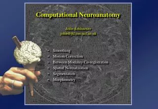
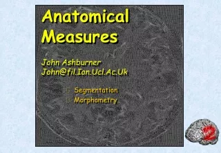
Voxel-Based Morphometry John Ashburner john@fil.ion.ucl.ac.uk. Functional Imaging Lab, 12 Queen Square, London, UK. Contents. Morphometry Volumes from deformations Serial scans Voxel-based morphometry Spatial normalisation in SPM2 Tissue Classification in SPM2 Unified Segmentation.

E N D
Voxel-Based MorphometryJohn Ashburnerjohn@fil.ion.ucl.ac.uk Functional Imaging Lab, 12 Queen Square, London, UK.
Contents • Morphometry • Volumes from deformations • Serial scans • Voxel-based morphometry • Spatial normalisation in SPM2 • Tissue Classification in SPM2 • Unified Segmentation
Deformation Field Original Warped Template Deformation field
Jacobians Jacobian Matrix (or just “Jacobian”) Jacobian Determinant (or just “Jacobian”) - relative volumes
Serial Scans Early Late Difference Data from the Dementia Research Group, Queen Square.
Regions of expansion and contraction • Relative volumes encoded in Jacobian determinants.
Late Early Late CSF Early CSF CSF “modulated” by relative volumes Warped early Difference Relative volumes
Late CSF - modulated CSF Late CSF - Early CSF Smoothed
Smoothing Each voxel after smoothing effectively becomes the result of applying a weighted region of interest (ROI). Before convolution Convolved with a circle Convolved with a Gaussian
Voxel-based Morphometry • Pre-process images of several subjects to highlight particular differences. • Tissue volumes • Use mass-univariate statistics (t- and F-tests) to detect differences among the pre-processed data (next week). • Use Gaussian Random Field Theory to interpret the blobs (next week).
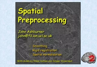
Contents • Morphometry • Spatial normalisation in SPM2 • Affine registration • Nonlinear registration • Tissue Classification in SPM2 • Unified Segmentation
Spatial Normalisation - Procedure • Begin with affine registration • Non-linear registration (about 1000 parameters) Affine registration Non-linear registration
Maximum a posteriori solution (global optimum) P(q|y) Local optimum Local optimum Value of q(in 1-D) Probabilities • P(q|y) = P(y|q) P(q) / P(y) • where • y is data • q is the estimated transform • Registration objective function is:E(q|y) = E(y|q) + E(q) + const • where E(*) = -log(P(*)) • E(y) is assumed constant
Gauss-Newton Optimisation • MAP solution is estimated by fitting a quadratic to E(q|y) at each iteration • Additional stability could be achieved by Levenberg-Marquardt approach.
Spatial Normalisation - Affine • The first part is a 12 parameter affine transform • Fits overall shape and size • Parallel lines remain parallel • Operations can be represented by: x1 = m11x0 + m12y0 + m13z0 + m14 y1 = m21x0 + m22y0 + m23z0 + m24 z1 = m31x0 + m32y0 + m33z0 + m34 • Algorithm simultaneously minimises • E(y|q) Mean-squared difference between template and source image • E(q) Squared distance between parameters and their expected values (regularisation)
Spatial Normalisation - Non-linear Deformations consist of a linear combination of smooth basis functions These are the lowest frequencies of a 3D discrete cosine transform (DCT) Algorithm simultaneously minimises • E(y|q) Mean squared difference between template and source image • E(q) Weighted squared magnitude of parameters
Spatial Normalisation - Overfitting Without regularisation, the non-linear spatial normalisation can introduce unnecessary warps. Affine registration. (2 = 472.1) Template image Non-linear registration without regularisation. (2 = 287.3) Non-linear registration using regularisation. (2 = 302.7)
Contents • Morphometry • Spatial normalisation in SPM2 • Tissue Classification in SPM2 • Gaussian mixture model • Including prior probability maps • Intensity non-uniformity correction • Unified Segmentation
Tissue Classification - Mixture Model • Intensities are modelled by a mixture of K gaussian distributions, parameterised by: • Means • Variances • Mixing proportions • Can be multi-spectral • Multivariategaussiandistributions
Tissue Classification - Priors • Overlay prior belonging probability maps to assist the segmentation • Prior probability of each voxel being of a particular type is derived from segmented images of 151subjects • Assumed to berepresentative • Requires initialregistration tostandard space
Tissue Classification - Bias Correction • A smooth intensity modulating function can be modelled by a linear combination of DCT basis functions
Tissue Classification - Algorithm Starting estimates for belonging probabilities based on prior probability images Compute cluster parameters from belonging probabilities and bias field Compute belonging probabilities from cluster parameters and bias field Compute bias field from belonging probabilities and cluster parameters Converged? No Yes Done
Spatial Normalisation using Tissue Classes • The “Optimised VBM” strategy Spatially Normalised MRI Template Original MRI Affine register Spatial Normalisation - writing Affine Transform Segment Grey Matter Spatial Normalisation - estimation Priors Deformation
Contents • Morphometry • Spatial normalisation in SPM2 • Tissue Classification in SPM2 • Unified Segmentation
Unified Segmentation • Circularity: • Registration is helped by tissue classification and bias correction. • Tissue classification is helped by registration and bias correction. • Bias correction is helped by registration and tissue classification. • The solution is to put everything in the same generative model. • A MAP solution is found by repeatedly alternating among classification, bias correction and registration steps. • Should produce “better” results than simple serial applications of each component.
Mixture of Gaussians (MOG) • Classification is based on a Mixture of Gaussians model (MOG), which represents the intensity probability density by a number of Gaussian distributions. • Data consists of I voxels, of intensity yi. • Each of K Gaussians is parameterised by its mixing proportion (gk), mean (mk) and variance (s2k). • The negative log-likelihood (E) is given by:
Modelling a Bias Field • A bias field is included, such that the required scaling at voxel i, parameterised by b, is ri(b). yr(b) r(b) y
Warped Prior Probabilities • Deformed prior probability images for each class are included, where the warps are parameterised by a. After warping, the value of the ith voxel of image k is qik(a). The prior probability of obtaining class k at voxel i, given parameters a and weights g is then: ICBM Tissue Probabilistic Atlas Images
The Extended MOG • By combining the modified P(k|q) and P(yi|k,q), the objective function becomes: • Bias and nonlinear deformations are parameterised by a linear combination of cosine transform bases, where a and b are the estimated coefficients.
Schematic of optimisation Repeat until convergence Hold a and b constant, and minimise E w.r.t. g, m and s2 - Differentiate E w.r.t. each parameter, and solve. - Requires substitution of current belonging probabilities at each iteration. Hold g, m, s2 and a constant, and minimise E w.r.t. b - Levenberg-Marquardt strategy, using dE/db and d2E/db2 Hold g, m, s2 and b constant, and minimise E w.r.t. a - Levenberg-Marquardt strategy, using dE/da and d2E/da2 end • Regularisation keeps deformations and bias smooth. • Properties of Kronecker tensor products used for speed.