Image Registration John Ashburner
660 likes | 819 Vues
Image Registration John Ashburner. Pre-processing Overview. Statistics or whatever. fMRI time-series. Template. Anatomical MRI. Smoothed. Estimate Spatial Norm. Motion Correct. Smooth. Coregister. Spatially normalised. Deformation. Contents. Preliminaries Smooth

Image Registration John Ashburner
E N D
Presentation Transcript
Pre-processing Overview Statistics or whatever fMRI time-series Template Anatomical MRI Smoothed Estimate Spatial Norm Motion Correct Smooth Coregister Spatially normalised Deformation
Contents • Preliminaries • Smooth • Rigid-Body and Affine Transformations • Optimisation and Objective Functions • Transformations and Interpolation • Intra-Subject Registration • Inter-Subject Registration
Smooth Smoothing is done by convolution. Each voxel after smoothing effectively becomes the result of applying a weighted region of interest (ROI). Before convolution Convolved with a circle Convolved with a Gaussian
Image Registration • Registration - i.e. Optimise the parameters that describe a spatial transformation between the source and reference (template) images • Transformation - i.e. Re-sample according to the determined transformation parameters
2D Affine Transforms • Translations by tx and ty • x1 = x0 + tx • y1 = y0 + ty • Rotation around the origin by radians • x1 = cos() x0 + sin() y0 • y1 = -sin() x0 + cos() y0 • Zooms by sx and sy • x1 = sx x0 • y1 = sy y0 • Shear • x1 = x0 + h y0 • y1 = y0
2D Affine Transforms • Translations by tx and ty • x1 = 1 x0 + 0 y0 + tx • y1 = 0 x0 + 1 y0 + ty • Rotation around the origin by radians • x1 = cos() x0 + sin() y0 + 0 • y1 = -sin() x0 + cos() y0 + 0 • Zooms by sx and sy: • x1 = sx x0 + 0 y0 + 0 • y1 = 0 x0 + sy y0 + 0 • Shear • x1 = 1 x0 + h y0 + 0 • y1 = 0 x0 + 1 y0 + 0
3D Rigid-body Transformations • A 3D rigid body transform is defined by: • 3 translations - in X, Y & Z directions • 3 rotations - about X, Y & Z axes • The order of the operations matters Translations Pitch about x axis Roll about y axis Yaw about z axis
Voxel-to-world Transforms • Affine transform associated with each image • Maps from voxels (x=1..nx, y=1..ny, z=1..nz) to some world co-ordinate system. e.g., • Scanner co-ordinates - images from DICOM toolbox • T&T/MNI coordinates - spatially normalised • Registering image B (source) to image A (target) will update B’s voxel-to-world mapping • Mapping from voxels in A to voxels in B is by • A-to-world using MA, then world-to-B using MB-1 • MB-1 MA
Left- and Right-handed Coordinate Systems • NIfTI format files are stored in either a left- or right-handed system • Indicated in the header • Talairach & Tournoux uses a right-handed system • Mapping between them sometimes requires a flip • Affine transform has a negative determinant
Optimisation • Image registration is done by optimisation. • Optimisation involves finding some “best” parameters according to an “objective function”, which is either minimised or maximised • The “objective function” is often related to a probability based on some model Most probable solution (global optimum) Objective function Local optimum Local optimum Value of parameter
Objective Functions • Intra-modal • Mean squared difference (minimise) • Normalised cross correlation (maximise) • Entropy of difference (minimise) • Inter-modal (or intra-modal) • Mutual information (maximise) • Normalised mutual information (maximise) • Entropy correlation coefficient (maximise) • AIR cost function (minimise)
Simple Interpolation • Nearest neighbour • Take the value of the closest voxel • Tri-linear • Just a weighted average of the neighbouring voxels • f5 = f1 x2 + f2 x1 • f6 = f3 x2 + f4 x1 • f7 = f5 y2 + f6 y1
B-spline Interpolation A continuous function is represented by a linear combination of basis functions 2D B-spline basis functions of degrees 0, 1, 2 and 3 B-splines are piecewise polynomials Nearest neighbour and trilinear interpolation are the same as B-spline interpolation with degrees 0 and 1.
Contents • Preliminaries • Intra-Subject Registration • Realign • Mean-squared difference objective function • Residual artifacts and distortion correction • Coregister • Inter-Subject Registration
Mean-squared Difference • Minimising mean-squared difference works for intra-modal registration (realignment) • Simple relationship between intensities in one image, versus those in the other • Assumes normally distributed differences
Residual Errors from aligned fMRI • Re-sampling can introduce interpolation errors • especially tri-linear interpolation • Gaps between slices can cause aliasing artefacts • Slices are not acquired simultaneously • rapid movements not accounted for by rigid body model • Image artefacts may not move according to a rigid body model • image distortion • image dropout • Nyquist ghost • Functions of the estimated motion parameters can be modelled as confounds in subsequent analyses
Movement by Distortion Interaction of fMRI • Subject disrupts B0 field, rendering it inhomogeneous • distortions in phase-encode direction • Subject moves during EPI time series • Distortions vary with subject orientation • shape varies
Correcting for distortion changes using Unwarp Estimate reference from mean of all scans. • Estimate new distortion fields for each image: • estimate rate of change of field with respect to the current estimate of movement parameters in pitch and roll. Unwarp time series. Estimate movement parameters. + Andersson et al, 2001
Contents • Preliminaries • Intra-Subject Registration • Realign • Coregister • Mutual Information objective function • Inter-Subject Registration
Inter-modal registration • Match images from same subject but different modalities: • anatomical localisation of single subject activations • achieve more precise spatial normalisation of functional image using anatomical image.
Mutual Information • Used for between-modality registration • Derived from joint histograms • MI= ab P(a,b) log2 [P(a,b)/( P(a) P(b) )] • Related to entropy: MI = -H(a,b) + H(a) + H(b) • Where H(a) = -a P(a) log2P(a) and H(a,b) = -a P(a,b) log2P(a,b)
Contents • Preliminaries • Intra-Subject Registration • Inter-Subject Registration • Normalise • Affine Registration • Nonlinear Registration • Regularisation • Segment • DARTEL
Spatial Normalisation - Procedure • Minimise mean squared difference from template image(s) Affine registration Non-linear registration
Spatial Normalisation - Templates T1 Transm T2 T1 305 T2 PD SS PD PET EPI Template Images “Canonical” images Spatial normalisation can be weighted so that non-brain voxels do not influence the result. Similar weighting masks can be used for normalising lesioned brains.
Spatial Normalisation - Affine • The first part is a 12 parameter affine transform • 3 translations • 3 rotations • 3 zooms • 3 shears • Fits overall shape and size • Algorithm simultaneously minimises • Mean-squared difference between template and source image • Squared distance between parameters and their expected values (regularisation)
Spatial Normalisation - Non-linear Deformations consist of a linear combination of smooth basis functions These are the lowest frequencies of a 3D discrete cosine transform (DCT) Algorithm simultaneously minimises • Mean squared difference between template and source image • Squared distance between parameters and their known expectation
Spatial Normalisation - Overfitting Without regularisation, the non-linear spatial normalisation can introduce unnecessary warps. Affine registration. (2 = 472.1) Target image Non-linear registration without regularisation. (2 = 287.3) Non-linear registration using regularisation. (2 = 302.7)
Contents • Preliminaries • Intra-Subject Registration • Inter-Subject Registration • Normalise • Segment • Gaussian mixture model • Intensity non-uniformity correction • Deformed tissue probability maps • DARTEL
Segmentation • Segmentation in SPM5 also estimates a spatial transformation that can be used for spatially normalising images. • It uses a generative model, which involves: • Mixture of Gaussians (MOG) • Bias Correction Component • Warping (Non-linear Registration) Component
Mixture of Gaussians (MOG) • Classification is based on a Mixture of Gaussians model (MOG), which represents the intensity probability density by a number of Gaussian distributions. Frequency Image Intensity
Belonging Probabilities Belonging probabilities are assigned by normalising to one.
Non-Gaussian Intensity Distributions • Multiple Gaussians per tissue class allow non-Gaussian intensity distributions to be modelled. • E.g. accounting for partial volume effects
Modelling a Bias Field • A bias field is modelled as a linear combination of basis functions. Corrected image Corrupted image Bias Field
Tissue Probability Maps • Tissue probability maps (TPMs) are used instead of the proportion of voxels in each Gaussian as the prior. ICBM Tissue Probabilistic Atlases. These tissue probability maps are kindly provided by the International Consortium for Brain Mapping, John C. Mazziotta and Arthur W. Toga.
Deforming the Tissue Probability Maps • Tissue probability images are deformed so that they can be overlaid on top of the image to segment.
Optimisation • The “best” parameters are those that minimise this objective function. • Optimisation involves finding them. • Begin with starting estimates, and repeatedly change them so that the objective function decreases each time.
Steepest Descent Start Optimum Alternate between optimising different groups of parameters
Spatially normalised BrainWeb phantoms (T1, T2 and PD) Tissue probability maps of GM and WM Cocosco, Kollokian, Kwan & Evans. “BrainWeb: Online Interface to a 3D MRI Simulated Brain Database”. NeuroImage 5(4):S425 (1997)
Contents • Preliminaries • Intra-Subject Registration • Inter-Subject Registration • Normalise • Segment • DARTEL • Flow field parameterisation • Objective function • Template creation • Examples
A one-to-one mapping • Many models simply add a smooth displacement to an identity transform • One-to-one mapping not enforced • Inverses approximately obtained by subtracting the displacement • Not a real inverse Small deformation approximation
DARTEL • Parameterising the deformation • φ(0)(x) = x • φ(1)(x) = ∫u(φ(t)(x))dt • u is a flow field to be estimated • Scaling and squaring is used to generate deformations. 1 t=0
Registration objective function • Simultaneously minimize the sum of: • Likelihood component • Drives the matching of the images. • Multinomial assumption • Prior component • A measure of deformation roughness • Regularises the registration. • ½uTHu • A balance between the two terms.
Likelihood Model • Current DARTEL model is multinomial for matching tissue class images. • Template represents probability of obtaining different tissues at each point. log p(t|μ,ϕ) = ΣjΣk tjk log(μk(ϕj)) t – individual GM, WM and background μ– template GM, WM and background ϕ– deformation
Grey matter Grey matter Grey matter Grey matter White matter White matter White matter White matter Simultaneous registration of GM to GM and WM to WM Subject 1 Subject 3 Grey matter White matter Template Subject 2 Subject 4
Template Initial Average Iteratively generated from 471 subjects Began with rigidly aligned tissue probability maps Used an inverse consistent formulation After a few iterations Final template