Medical Image Registration
1.09k likes | 1.74k Vues
Medical Image Registration. Kumar Rajamani. Registration . Spatial transform that maps points from one image to corresponding points in another image. Time axis : aging , development …. z. Cross-subject, same modality. …. y. x. Anatomy. …. Label. …. Same subject, cross modality.

Medical Image Registration
E N D
Presentation Transcript
Medical Image Registration Kumar Rajamani
Registration • Spatial transform that maps points from one image to corresponding points in another image
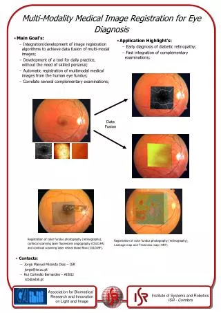
Timeaxis: aging, development… z Cross-subject, same modality … y x Anatomy … Label … Same subject, cross modality Function … … … … Pathology, Histology… Image Registration • Data Fusion • Atlases for population studies • Motion Correction for image reconstruction • Surgery Planning Common coordinate system
Rigid Deformable Similarity Rigid + Scale Affine Scale / Skew Example Registration Transformations Original
Image comparison Registered moving image Difference before registration Difference after registration
After Registration Before Registration *GE Owned B-Splines based Registration
Registration Criteria • Landmark-based • Features selected by the user • Segmentation-based • Rigidly or deformably align binary structures • Intensity-based • Minimize intensity difference over entire image
Spatial Transformation • Rigid • Rotations and translations • Affine • Also, skew and scaling • Deformable • Free-form mapping
Registration framework pieces • 2 input images, fixed and moving • Metric - determines the “fitness” of the current registration iteration • Optimizer - adjusts the transform in an attempt to improve the metric • Interpolator - applies transform to image and computes sub-pixel values
optimizer metric transform Registration — General Problem Common coordinate system Domain of an individual subject f m Problem: Find transform T such that image f[p] matches m[T(p)] Interpolate
Transforms • x’=T(x|p)=T(x,y|tx,ty,θ) • Goal: Find parameter values that optimize image similarity metric
Optimizer • Often require derivative of image similarity metric (S)
Understanding the Transform Jacobian • J shows how changing p shifts a transformed point in the moving image space. • This allows efficient use of a pre-computed moving-image gradient to infer changes in corresponding-pixel intensities for changes in p • Now we can update dS/dp by just updating J
Transforms • Before we discuss specific transforms, let’s discuss the… • Fixed Set = the set of points (i.e. physical coordinates) that are unchanged by the transform • The fixed set is a very important property of a transform
Identity Transform • Maps every point to itself • Only used for testing • Fixed set = everything (i.e., the entire space)
Translation Transform • Fixed set = empty set • Translation can be closely approximated by: • Small rotation about distant origin, and/or… • Small scale about distant origin • Both of these do have a fixed point • Optimizers will frequently (accidently) do translation by using either rotation or scale • This makes the optimization space harder to use • The final transform may be harder to understand
Translation Transform • Fixed set is an empty set
Scaling Transform • Isotropic vs. anisotropic • Fixed set is the origin of the coordinates C C
2D Rotation Transform • Rotation transforms are typically specific to either 2D or 3D • Fixed set = origin = “center” = C C C
Translation Rotation Scaling Transforms • Affine Transform • S=Id reduces to Rigid case, (e.g. Head motion correction) • Affine Transforms also encode scale/skew factors Original Rigid
Optimization • Search for value of θ that minimizes cost function S • Gradient descent algorithm • Update of parameter • G is the variation from the gradient of the cost function • is step length of algorithm
Sequence of translations and metric values at each iteration of the optimizer
Scaling, Rotation,Translation • P=arbitrary point • C=fixed point of transformation • D=scaling factor • Θ=rotation angle • P and C are complex numbers (x+iy) or reiθ • Store derivates of P in Jacobian matrix for optimizer • Rigid if D=1, otherwise similarity transform
Affine Transformation • Collinearity is preserved • x’=A x + T • A is a complex matrix of coefficients • With fixed point • x’=A (x–C) + C • A is optimized similar to the scaling factor
Quaternions • Quotient of two vectors • Q= A / B • Operator that produces second vector • A= Q B • Represents orientation of one vector with respect to another, as well as ratio of their magnitudes • Versor-rotates vector • Tensor-changes vector magnitude
Scalars and Versors • Quaternion represented by 4 numbers • Versor • Direction – parallel to axis of rotation • Rotation angle • Norm – function of rotation angle • Tensor • Magnitude
Rigid Transform in 3D • Use quaternions instead of phasors • P’=V*(P-C)+C • P’=V*P+T, T=C-V*C • P=point, V=Versor, T=Translation, C=fixed point • Transform represented by 6 parameters • Three numbers representing versor • Three components of fixed coordinate system
Image Interpolators • 2 functions • Compute interpolated intensity at requested position • Detect whether or not requested position lies within moving-image domain
Nearest Neighbor • Uses intensity of nearest grid position • Computationally cheap • Doesn’t require floating point calculations
Linear Interpolation • Computed as the weighted sum of 2n-1 neighbors • n=dimensionality of image • Weighting is based on distance between requested position and neighbors
B-spline Interpolation • Intensity calculated by multiplying B-spline coefficients with shifted B-spline kernels • Higher spline orders require more pixels to computer interpolated value • Third-order B-spline kernels typically used because good tradeoff between smoothness and computational burden
Metrics • Scalar function of the set of transform parameters for a given fixed image, moving image, and transformation type • Typically samples points within fixed image to compute the measure
Mean Squares • Mean squared difference over all the pixels in an image • Intensities are interpolated for the moving image • For gradient-based optimization, derivative of metric is also required
Mean Squares • Optimal value of zero • Interpolator will affect computation time and smoothness of metric plot • Assumes intensity representing the same homologous point is in both images • Images must be from same modality
Mean Squares Smoothness affected by interpolator
Normalized Correlation • Computes pixel-wise cross-correlation between the intensity of the two images, normalized by the square root of the autocorrelation of each image • For two identical images, metric =1 • Misalignment, metric <1
Normalized Correlation • -1 added for minimum-seeking optimizers
Difference Density • Each pixel’s contribution is calculated using bell-shaped function • f(d) has a maximum of 1 at d=0 and minimum of zero at d=+/-infinity • d is difference in intensity b/w F and M
Multi-modal Volume Registration by Maximization of Mutual InformationWells W, Viola P, Atsumi H, Nakajima S, Kikinis R
Registering Images from Same Modality • Typical measure of error is sum of squared differences between voxels values • This measure is directly proportional to the likelihood that the images are correctly registered • Same measure is NOT effective for images of different modalities
MI Inputs Figure 8.9 from the ITK Software Guide v 2.4, by Luis Ibáñez, et al. T1 MRI Proton density MRI
Relationship Between Images of Different Modalities • Example: We should be able to construct a function F() that predicts CT voxel value from corresponding MRI value • Registration could be evaluated by computing F(MR) and comparing it to the CT image • Via sum of squared differences (or correlation) • In practice, this is a difficult and under-determined problem