Download
1 / 28
280 likes | 312 Vues
Explore innovative strategies and protocols to improve throughput in clockless pipelines while maintaining low latency. Discover Dual-Rail and Single-Rail signaling designs like LP3/1, LP2/2, and LP2/1 for early evaluation and completion detection. Compare their cycle times and efficiencies over traditional PS0 pipelines.

E N D
Clockless Logic:Dynamic Logic Pipelines (contd.) Drawbacks of Williams’ PS0 Pipelines Lookahead Pipelines
Drawbacks of PSO Pipelining • Poor throughput: • long cycle time: 6 events per cycle • data “tokens” are forced far apart in time • Limited storage capacity: • max only 50% of stages can hold distinct tokens • data tokens must be separated by at least one spacer Our Research Goals: address both issues • still maintain very low latency
Recent Approaches 3 novel styles for high-speed async pipelining: • “Lookahead Pipelines” (LP) [Singh/Nowick, Async-00] • “High-Capacity Pipelines” (HC) [Singh/Nowick, WVLSI-00] • MOUSETRAP Pipelines [Singh/Nowick, TAU-00] Goal:significantly improve throughput of PS0 Two Distinct Strategies: • LP: introduce protocol optimizations • “shave off” components from critical cycle • HC: fundamentally new protocol • greater concurrency: “loosely-coupled” stages
Outline Dynamic circuit style Static circuit style • New Asynchronous Pipelines: • Lookahead Pipelines (LP) • High-Capacity Pipelines (HC) • MOUSETRAP Pipelines
Lookahead Pipelines: Strategy #1 Use non-neighbor communication: • stage receives information from multiple later stages • allows “early evaluation” Benefit: stage gets head-start on next cycle
Lookahead Pipelines: Strategy #2 Use early completion detection: • completion detector moved before stage (not after) • stage indicates“early done”in parallel with computation early completion detector Benefit: again, stage gets head-start on next cycle
Lookahead Pipelines: Overview 5 New Designs: • “Dual-Rail” Data Signaling: • LP3/1:“early evaluation” • LP2/2:“early done” • LP2/1:“early evaluation” + “early done” • “Single-Rail” Bundled-Data Signaling: • LPSR2/2:“early done” • LPSR2/1:“early evaluation” + “early done”
Dual-Rail Design #1: LP3/1 Optimization = “early evaluation” • each stage has two control inputs: from stages N+1 and N+2 Idea: shorten precharge phase • terminate precharge early: when N+2 is done evaluating PC Eval Data in Data out N N+1 N+2 Completion Detector ProcessingBlock From N+2
LP3/1 Protocol New! 4 3 N+1 indicates “done” 3 1 2 Enables “early evaluation!” • PRECHARGEN:when N+1 completes evaluation • EVALUATEN:whenN+2completes evaluation N+2 indicates “done” N N+1 N+2 N+2 evaluates N evaluates N+1 evaluates
LP3/1: Comparison with PS0 indicates “done” Enables “early evaluation!” 4 3 evaluates evaluates evaluates EVALUATE N: when N+2 completes evaluation PRECHARGE N: when N+1completes evaluation indicates “done” EVALUATE N: when N+1 completes precharging 5 4 6 3 1 2 3 3 1 2 evaluates evaluates evaluates N N+1 N+2 LP3/1 Only 4 events in cycle! N N+1 N+2 PS0 6 events in cycle
LP3/1 Performance 4 3 1 2 Cycle Time = saved path Savings over PS0:1 Precharge + 1 Completion Detection
LP3/1: Inside a Stage “old Eval” PC (From Stage N+1) Eval (From Stage N+2) “early Eval” NAND Merging 2 Control Inputs: A NAND gate merges2 control inputs: • Precharge whenPC=1(and Eval=0) • Evaluate “early”whenEval=1(or PC=0) • Problem: “early”Eval=1 is non-persistent! • may be de-asserted before stage completes evaluation!
LP3/1 Timing Constraints: Example PC (From Stage N+1) Eval (From Stage N+2) NAND Observation:PC=0soon after Eval=1, and is persistent Solution:no change! use PC as safe“takeover”for Eval! Timing Constraint:PC=0must arrivebeforeEval de-asserted • simple one-sided timing requirement • other constraints as well… all easily satisfied in practice Problem (cont.):“early”Eval=1 non-persistent
Dual-Rail Design #2: LP2/2 Optimization = “early done” • Idea: move completion detector beforeprocessing block • stage indicates when“about to”precharge/evaluate “early” Completion Detector “early done” Data in Data out Processing Block
LP2/2 Completion Detector PC bit0 bitn bit1 OR OR OR Done C + + + Modified completion detectors needed: • Done=1 when stage starts evaluating, and inputs valid • Done=0 when stage starts precharging • asymmetric C-element
LP2/2 Protocol “early done” of N+1 eval 2 3 “early done” of N+1 prech 4 “early done” of N+2 eval 1 2 3 Completion Detection: performedin parallel with evaluation/precharge of stage N N+1 N+2 N evaluates N+1 evaluates
LP2/2 Performance 3 Cycle Time = 4 1 2 LP2/2 savings over PS0: 1 Evaluation + 1 Precharge
Dual-Rail Design #3: LP2/1 Hybrid of LP3/1 and LP2/2… Combines: • early evaluationof LP3/1 • early doneof LP2/2 Cycle time:Best of our dual-rail lookahead pipelines…
Dual-Rail Design #3: LP2/1 Cycle Time = Hybrid of LP3/1 and LP2/2. Combines: • early evaluation of LP3/1 • early done of LP2/2
Lookahead Pipelines: Overview 5 New Designs: • “Dual-Rail” Data Signaling: • LP3/1:“early evaluation” • LP2/2:“early done” • LP2/1:“early evaluation” + “early done” • “Single-Rail” Bundled-Data Signaling: • LPSR2/2:“early done” • LPSR2/1:“early evaluation” + “early done”
Single-Rail Design: LPSR2/1 delay delay delay • “Ack” to previous stages is “tapped off early” • once in evaluate (precharge), dynamic logic insensitive to input changes Derivative of LP2/1, adapted to single-rail: • bundled-data: matched delays instead of completion detectors
Inside an LPSR2/1 Stage PC (From Stage N+1) Eval (From Stage N+2) matcheddelay “ack” NAND “req” out done “req” in data out data in aC + • “done” generated by an asymmetric C-element • done=1 when stage evaluates, and data inputs valid • done=0 when stage precharges PC and Eval are combined exactly as in LP3/1
LPSR2/1 Protocol N+1 indicates “done” N+2 indicates “done” 2 3 2 1 N+1 evaluates N+2 evaluates Cycle Time = N N+1 N+2 N evaluates
Results Designed/simulated FIFO’s for each pipeline style Experimental Setup: • design: 4-bit wide, 10-stage FIFO • technology: 0.6 HP CMOS • operating conditions: 3.3 V and 300°K
Comparison with Williams’ PS0 • LP2/1: >2X faster than Williams’ PS0 • LPSR2/1: 1.2 Giga items/sec dual-rail single-rail
Comparison: LPSR2/1 vs. Molnar FIFO’s LPSR2/1 FIFO: 1.2 Giga items/sec Adding logic processing to FIFO: • simply fold logic into dynamic gate little overhead Comparison with Molnar FIFO’s: • asp* FIFO: 1.1 Giga items/sec • more complex timing assumptions not easily formalized • requires explicit latches, separate from logic! • adding logic processing between stages significant overhead • micropipeline: 1.7 Giga items/sec • two parallel FIFO’s, each only 0.85 Giga/sec • very expensive transition latches • cannot add logic processing to FIFO!
Practicality of Gate-Level Pipelining fan-out=2 done comp. det. fan-in = 2 datapath width = 32 dual-rail bits! When datapath is wide: • Can often split into narrow “streams” • Use “localized” completion detector for each stream: • need to examine only a few bits small fan-in • send “done” to only a few gates small fan-out • comp. det. fairly low cost!
Conclusions Introduced several new dynamic pipelines: • Use two novel protocols: • “early evaluation” • “early done” • Especially suitable for fine-grain (gate-level) pipelining • Very high throughputs obtained: • dual-rail:>2X improvement over Williams’ PS0 • single-rail:1.2 Giga items/second in 0.6 CMOS • Use easy-to-satisfy, one-sided timing constraints • Robustly handle arbitrary-speed environments • overcome a major shortcoming of Williams’ PS0 pipelines Recent Improvement: Even faster single-rail pipeline (WVLSI’00)