Download
1 / 50
500 likes | 532 Vues
Explore instant stereoscopic tomography of active regions in 3D coronal loops for electron density and temperature measurements using STEREO spacecraft. Conduct 3D reconstructions and study loop geometries with detailed stereo error calculations. Use hydrostatic modeling for loop height determination and temperature measurements with background subtraction and filter analysis. Understand loop structures and dynamics through innovative tomographic approaches.

E N D
Instant Tomography of Active Regions Markus J. Aschwanden Jean-Pierre Wuelser, Nariaki Nitta, & James Lemen (LMSAL) STEREO Science Working Group Meeting Old Pasadena, CA, February 3-5, 2009 http://www.lmsal.com/~aschwand/ppt/2009_SWG_Pasasena_Tomo.ppt
Content of talk : Stereoscopic reconstruction of 3D geometry of coronal loops Electron density and temperature measurements Instant stereoscopic tomography of active regions (ISTAR) Relevant Publications: -Aschwanden, Wuelser, Nitta, & Lemen 2008: “First 3D Reconstructions of Coronal Loops with the STEREO A+B Spacecraft: I. Geometry (2008, ApJ 679, 827) II. Electron Density and Temperature Measurements (2008, ApJ 680, 1477) III. Instant Stereoscopic Tomography of Active regions (2008, ApJ 694, Apr 1 issue)
May 2007 Nov 2007 STEREO A-B separation angles (2007 is prime phase for small-angle stereoscopy) Date B (deg East) A(deg West) A-B(deg separation) 2007-Jan-1 0.151 0.157 0.009 2007-Feb-1 0.167 0.474 0.623 2007-Mar-1 0.169 1.061 1.229 2007-Apr-1 0.740 2.307 3.032 2007-May-1 1.888 4.213 6.089 2007-Jun-1 3.762 6.843 10.600 2007-Jul-1 6.196 9.810 16.004 2007-Aug-1 9.211 12.975 22.186 2007-Sep-1 12.525 15.871 28.396 2007-Oct-1 15.764 18.127 33.891 2007-Nov-1 18.830 19.744 38.574 2007-Dec-1 21.216 20.660 41.876 2008-Jan-1 22.837 21.182 44.018
2007 May 9, 20:40:45 UT, 171 A, STEREO-A, EUVI Target AR in A
2007 May 9, 20:41:30 UT, 171 A, STEREO-B Target AR in B
Coaligned STEREO image pair A+B with FOV of AR Highpass-filtered STEREO image pair A+B
Image Highpass-Filtering and Loop Definition Best S/N ratio, but widest loops Unfiltered image (100% flux) Higphass filter (w<21 pixel) Lowest S/N ratio, but narrowest loops Highpass filter (w<3 pixel; 4% flux) Highpass filter (w<7 pixel)
With a highpass filter we enhance the finest loop strands, but EUVI has a spatial resolution of 3.5” (2.2 EUVI pixels = 2500 km), and thus the finest structures seen with EUVI probably correspond to “composite” loops. TRACE found elementary (isothermal) loops for w<1500 km Simultaneous images recorded in EUV in near-identical temperature filters (e.g., TRACE 171 A vs CDS Mg IX, ~ 1.0 MK) reveal that a loop system observed with CDS (with a spatial resolution of ~4” pixel) is composed of at least 10 loop strands when imaged with TRACE (with a pixel size of 0.5” and spatial resolution of ~1”). Concept of elementary loop strands and composite loops:
The fact that all analyzed loops in EUVI have a diameter close to the spatial resolution of EUVI indicates that they are unresolved and have smaller real diameters: d<2.5 Mm
Observables: dA, dB, A, B, A, B, sep Trigonometric relations: Calculated parameters: x, y, z, r, h
Stereoscopic 3D Reconstruction z • - Manual clicking on 4-8 loop positions • in STEREO-A image (xA,yA) • Manual clicking on 4-8 loop positions • in STEREO-B image (xB, yB) • Calculating (x,y,z) 3D coordinates • from stereoscopic parallax • Calculate stereoscopic error • for each loop point z z • Weighted polynomial fit z(s) • (2nd-order) with s’ the projected • loop length coordinate s in [x,y] plane • Stereoscopic error in z-coordinate: y Error=1/2 pixel in NS direction infinite in EW direction x
Highpass filter: subtract image smoothed with 3x3 boxcar Highpass filter: subtract image smoothed with 5x5 boxcar
3D projections of loop geometries: [x,y] --> [x,z],[y,z] Color: blue=short loops red=midsize loops yellow=long loops white=longest loop
View in NS projection with errors of heights
Circularity ratio: C(s) = R(s)/rcurv Coplanarity ratio: P(s)=yperp(s)/rcurv
Hydrostatic Modeling The true vertical scale height can only be determined from proper (stereoscopic) 3D reconstruction of the loop geometry: --> Tests of hydrostatic equilibrium vs. super-hydrostatic dynamic states
Entire loops are only visible because of the large inclination angles: ~ 51 … 73 deg so that their apex is in an altitude of less than about a hydrostatic scale height.
The height limit of detectable loops is given by the dynamic range of the (hydrostatic) emission measure contrast:
Density and Temperature Measurements The determination of the density and temperature of a loop can only be done after background subtraction. The finest loop strands have typically a loop-related EUV flux of < 10%, and thus suitable background modeling in all 3 temperature filters is required.
Loop cross-section profiles are extracted from image. Background modeling with cubic polynomial interpolation.
Temperature response functions of EUVI, A+B Filter ratios for Gaussian DEM distributions: Triple-filter analysis: forward-fitting of EMp, Tp, DEM:
Example of simulating 3 iso-thermal (Ti=1.0, 1.4, 2.0 MK) loop cross-sections EM(x) with Gaussian profile, scaled with the TRACE response functions Rw(T) that yields in each case the profiles Fw(x)=EM(x) * Rw(Ti) seen in the three filters (w=171, 195, 284 A).
Input: background-subtracted loop flux profiles Output: Electron density and temperature profiles
The advantage of STEREO is that a loop can be mapped from two different directions, which allows for two independent background subtractions. This provides an important consistency test of the loop identity and the accuracy of the background flux subtraction. A B F b F a x x Consistency check: Is F_a = F_b ?
Consistency test between STEREO A+B: Two independent background subtractions from identical loop seen from two different angles: Do we arrive at the same loop widths, densities, and temperatures ?
A colored temperature map of 30 loops with temperatures in the range of T=0.8-1.5 MK The hottest loops tend to be the smallest loops, located in the center of the active region.
The density profiles n(h) are consistent with the gravitational stratification of hydrostatic loops, n(h) = nbase exp(-h/T) defined by the temperature scale heights T and stereoscopically measured from the height profiles h(s).
Overpressure p/pRTV > 1 RTV pressure p/pRTV=1 The observed densities are not consistent with hydrostatic equilibrium solutions, but rather display the typical overpressures of loops that have been previously heated to higher temperatures and cool down in a non-equilibrium state, similarly to earlier EIT and TRACE measurements.
Hydrodynamic simulations of impulsively heated loops reveal : (i) an underpressure (compared with the RTV hydrostatic equilibrium solution) during the heating phase, (ii) an RTV (energy balance) equilibrium point at the density peak, and (iii) an increasing overpressure during the cooling phase, approximately following the Jakmiec relation T(t)~n(t)2
EUV loops are generally observed during the non-equilibrium cooling phase, where they exhibit a high overpressure. The previously hotter temperature during the heating phase can be detected in soft X-rays. (see Winebarger, Warren, & Mariska 2003).
Image Preprocessing: (3) Multi-filter loop tracing 171 A 195 A 284 A
3D Field Interpolation Skeleton field = triangulated 3D loops 3D field vector = weighted 3D- interpolation
3D field interpolation Skeleton field of 100 triangulated loops with polarity assignment according to proximity to photospheric dipole config.
Tomographic volume rendering
Observations: 3 filter images Model: ~7000 loops (forward-fitting of fluxes)
3 different views
Statistical distributions of forward-fitted physical parameters
Differential emission measure distribution of forward-fitted AR model (with & without tapering of loop footpoints)
Forward-fitted AR model yields super-hydrostatic loops for T<3 MK
Density model Temperature model of forward-fit
Conclusions 2007 is the prime mission time for classical stereosocopy with small separation angles (<400). SDO will be launched when STEREO has very large separation not suitable for stereoscopy. The stereoscopic triangulation provides the 3D loop coordinates [x,y,z], the inclination angle of loop planes that is important for modeling the (hydrostatic) gravitational stratification, the LOS angle and projected loop widths for inferring the electron density. The dual stereoscopic view provides two independent background subtractions which yields a self-consistency test for the inferred physical loop parameters The 3D (x,y,z) coordinates of loops provide the the most accurate geometric constraints for magnetic modeling of active regions. Using stereoscopically triangulated loops as a skeleton, a 3D field can be interpolated and filled with plasma to produce a volumetric rendering of an active region, aiding forward-fitting in other wavelengths.