Tomography
Tomography. The Radon transform is the key technology in CAT scanning, now used in every hospital since 1972. Nowadays the research frontier has shifted to MRI= magnetic resonance imaging. I will discuss both.

Tomography
E N D
Presentation Transcript
Tomography • The Radon transform is the key technology in CAT scanning, now used in every hospital since 1972. Nowadays the research frontier has shifted to MRI= magnetic resonance imaging. I will discuss both. • An X-ray moves through an object of density f(x,y) at the point (x,y). It is absorbed or deflected with probability f(x,y) ds where ds is the element of length along a line, L, through (x,y). The chance it goes all the way along L is exp(-Pf(L) ) where
Why line integrals? • Beer’s law says that the log of the ratio of input to detected X-ray photons is proportional to the line integral of the density along the straight line path of the X-ray beam. • If an X-ray passes through an object of density f(s) at the point s, then the probability that it gets to s+ds given that it gets to s is 1-f(s) ds +o(ds). • Multiplying all these probabilities proves Beer’s law. So the Radon transform, Pf(L), the line integral of a object with density (gm/cc), f(x,y) can be measured. Radon’s theorem does the rest.
Rando phantom • He has no neck. He is used to calibrate scanners. Note that X-ray images are better for finding cavities than to study brain tumors. Why is this?
Interior tissue density • Fat = .9 • Bone = 2 • Water = 1 • Blood = 1.05 • Tumor = 1.03 • Gray matter = 1.02
First commercial CAT scanner EMI 1972 Godfrey Hounsfield • It measured one line integral at a time. The X-ray source is visible at the bottom, there is a detector at the top. It measured 100 line integrals and then rotated 1 degree and went back.
Anatomical “phantom” model Hounsfield invented tomography but didn’t think of using an anatomical model. This idea turned out useful. The line integrals can be calculated exactly. Errors in algorithm can be separated from errors due to noise in data.
The density values are chosen • Note the “skull”, “ventricles”, “tumors” Seems pretty silly, but I got very lucky with this idea as we’ll see.
The line integrals of the phantom • If the line misses the head the integral is zero. The small “tumors” contribute only to the 4th decimal place. Need many projections.
How to invert the Radon transform, ie “reconstruct” • The Fourier transform of the projection is equal to the two-dimensional Fourier transform of the object. Thus we know the Fourier transform of f. Now the Fourier inversion formula gives f
Derivative of the Hilbert transform operator In polar coordinates The Jacobian is |r|, and the product of f ^ with • |r| = (ir)( -i sgn(r)) • ir = derivative • -isgn(r) = Hilbert transform
What is the contribution from each line integral to the final reconstruction? • It’s a linear operator, f(x,y) = sum over L of c(L,(x,y) ) Pf(L), and we need only to know the coefficients c(L,x,y) of the inverse. These depend only on the distance from (x,y) to L. The filter function is the function of the distance. • It’s known as the Shepp-Logan filter. Many other filters would be as good.
The first 60 back-projected convolutions • These are the first 60 • Projections + convolutions
Convoluted backprojections 60-120 • These are the accumulated next 60 convoluted backprojections.
Convoluted backprojections 120-180 • After 180 backprojected convolution the reconstruction (upper left image) is complete.
Fourier reconstruction • Note streak artifacts outside the skull. Why are they present? • If God made us with the skull at the center of our brain and the brain on the outside CAT scanning would be much less useful.
Artifact due to an error in one line integral • Shows the filter’s contribution. But each line integral contributes to the whole reconstruction.
Old tomography • Simple backprojection with no filtering. Dates back to 1932 but never caught on. Not quite good enough to be useful.
Filtering allows cancellation • Old tomography gives not f(x,y) but f * (1/r). • Filtering removes the 1/r and gives back f(x,y) after accumulating the backprojections.
Note the accuracy • Except for some averaging this gives back the actual values chosen in the phantom 1.02 • The value in the tumor was 1.03, gray matter was 1.02.
Hounsfield’s reconstruction • Note the white just inside the skull. Is it real? It must be an artifact. It wasn’t in the original phantom. Lucky me. Hounsfield’s algorithm was iterative like Gauss-Seidel.
Later reconstruction by EMI • Much better, but still artifacted. This one was due to another engineer at EMI , Christopher Lemay. • Lemay could not convince Hounsfield to use a formula. However he did not use the Fourier approach either but a different one where there was no choice of filter.
Can use to set thresholds • CAT measurements of line integrals are accurate to .1%. f(x,y) is reconstructed to .5% • Radon inversion is a singular integral operator but it can be done practically as we see here.
CAT is sensitive to consistent errors in the 80th line integral • Some later CAT scanner designs allowed the detectors to rotate with the tube. These were subject to circle artifacts. • The 4th generation design avoided this problem but ASE lost to GE.
Amer Sci Eng’g 1974 600 detectors • The 4th generation design. Stationary detectors.
Some bad news • For every finite n, it is not enough to know n projections. There are invisible functions. In fact for every 0 < f < 1 there is a g = 0,1 with the same line integrals as f in the n directions. • Can CAT scanners be?
Coronal view • Can see ventricles • Not ellipses, alas.
Can use for the rest of the body too, but less useful • The fact that interior head tissue is nearly all the same becomes an advantage.
What is this body part? • Keep your guesses clean.
Lungs and chest • Note the rings in the board. This was an early test case at ASE.
Industrial application • Delamination in exit cone of rocket engine NASA
Simulation of the NASA situation • Even small delaminations can be found thanks to the streak artifacts we saw outside the skull.
Limited angle tomography • Can one do tomography with only 160 degrees of projections?
Best we could do • Judged not good enough for the application to fast CAT scanning • Probably not a good research problem. Analytic continuation is involved.
New topics • Emission tomography; PET, SPECT • The subject ingests a radio-pharmaceutical which moves under metabolic action to the place where the body’s chemistry needs it. It emits radiation which is measured. One can use a Poisson model of radiation which has no errors and attempt to find the maximum likelihood distribution that makes the observed photon counts in the detectors most likely. The problem with this technology is that it is too slow to be used to study fast mental processes.
Emission scanner PET • Gets lower resolution than CAT but it is more effective than CAT for metabolism studies. CAT cannot do metabolism at all. • CAT measures electron density.
Functional Magnetic Resonance Imaging • A hydrogen atom acts like a compass needle in a magnetic field and oscillates (spins) with a frequency proportional to field strength. Its spectrum changes with the local surrounding atoms and so magnetic resonance can be used for spectroscopy. In particular, oxy and deoxy hemoglobin can be distinguished by measuring their resonances due to the fact that the nearby oxygen atom changes slightly the rate of spin also due to the iron atom nearby. The possibility of this was pointed out by Pauling but Seiji Ogawa did it.
Magnetic Resonance Imaging • Paul Lauterbur made the magnetic field have a gradient so that the spins at different points would be separated. The spins induce an electrical current in a pick-up coil surrounding the subject. In this way if the local spin density at (x,y,z) is f(x,y,z) then • The current induced in the coil is called the free induction decay signal and is
Simple Fourier inversion • The current induced in the coil is thus the Fourier transform of the hydrogen spin density. Choosing different gradients (a,b,c) allows the Fourier transform to be measured at many points in k-space = Fourier space and the spin density f(x,y,z) can be obtained by direct Fourier inversion. This is standard MRI. I want to discuss a sub-topic, functional MRI.
Functional MRI • When you are thinking about lunch, which part of your brain is active? When you are instantaneously recognizing Monica Lewinsky, how is this done? • In fMRI, the difference of the spin density pre and post task is taken. This allows one to distinguish oxy and deoxy hemoglobin. But this has to be done in real time or we will never be able to see where the image of Monica is stored etc. How to sample the Fourier transform of the difference in real time. It costs 1 ms to sample f^(k) at one k.
Space-time trade off • We need good time resolution and are willing to give up spatial resolution if necessary. This can be done using the uncertainly principle analog. Suppose we measure the Fourier transform of the spin density on a small subset of Fourier or k-space. Then we can use the Parseval identity
Prolate spheroidal wave functions • We want to choose a phi^(k) that vanishes except on a small set A of k’s. • Then the right side is known if we only measure f ^ on A . This takes only 50 ms if A is small. • We also want to choose phi^ so that in brain space phi is compactly supported. The uncertainty principle says that if phi^ is compactly supported then phi cannot be. There is a MOST compactly supported phi though say for a sphere A in an L2 sense, maximizing the L2 integral over a region in brain space given that the L2 norm of phi is one.
The trajectory of the k-space measurements of f^(k) • The best region A in k-space is a sphere of low spatial frequencies, which is at first surprising. One might think one should try to sample k-space sparsely. We take A to be a small sphere. We then have to loop through A with a space-filling path along which we take our measurements of f^(k). • Which path to choose?
Ball of yarn 1 • One ball of yarn trajectory
Ball of yarn 2 • Second ball of yarn trajectory
How to choose the best trajectory? • The first trajectory seems to be more space-filling but it is also more complicated. A still loosely formulated problem is how to choose a curve which is most uniformly dense in a sphere. In 2D people use an Archimedean spiral but there are several natural generalizations to 3D. Best? Hector?