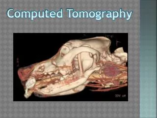
Computed Tomography
Computed Tomography. Tomos = slice. CT scan. Mathematical idea developed by Radon in 1917 Cormack did the instrumentation research 1963 published it A practical x-ray CT scanner was built by Hounsfield. When was the first computer introduced in laboratories?. The main idea.

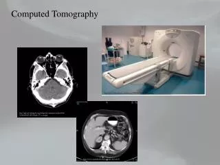
Computed Tomography
E N D
Presentation Transcript
Computed Tomography Tomos = slice
CT scan • Mathematical idea developed by Radon in 1917 • Cormack did the instrumentation research 1963 published it • A practical x-ray CT scanner was built by Hounsfield. When was the first computer introduced in laboratories?
The main idea Reconstruct the image of a non uniform sample using its x-ray projection at different angles
The main idea Reconstruct the image of a non uniform sample using its x-ray projection at different angles
The main idea Reconstruct the image of a non uniform sample using its x-ray projection at different angles
The main idea Reconstruct the image of a non uniform sample using its x-ray projection at different angles
The main idea Reconstruct the image of a non uniform sample using its x-ray projection at different angles
The main idea Reconstruct the image of a non uniform sample using its x-ray projection at different angles
Projection Radon transform
Inverse back-projection is used to reconstruct the original image from the projected image
CT images • Maps of relative linear attenuation of tissue • µ relative attenuation coefficient is expressed in Hounsfield units (HU) also known as CT numbers • HUx = 1000.(µx - µwater)/µwater • HUwater = 0 • HU depends on photon energy
CT images • FOV (field of view) Diameter of the region being imaged (head 25 cm) • Voxel Volume element in the patient • Pixel area x slice thickness
CT scan generations • 1st generation • Translate rotate, pencil beam • 2nd generation • Translate rotate, fan beam • 3rd generation • Rotate rotate, fan beam • 4th generation • Rotate, wide fan • 5th generation • Fixed array of detectors
X-ray tube • High voltage xray tubes • For large focal spots (1mm) ->high power (60kW), smaller spots (0.5 mm) low power rating (below 25kW) • Copper and aluminum filters used for beam hardening effect • Collimators both in x ray tube and detector
Detectors • Measure radiation through patient • High xray efficiency • Scintillation • Crystals produce visible range photons coupled with PMT • Xenon gas ionization detector • Gas chamber anode and cathode at potential. Used in 3rd gen., stable.
CT Image Reconstruction
CT • Please read Ch 13. • Homework is due 1 week from today at 12 pm.
Tomographic reconstruction detectors = 0o
The main idea detectors = 20o
The main idea detectors = 90o Reconstruct the image of a non uniform sample using its x-ray projection at different angles
The Sinogram Projection angle • • = 0 • • Detectors position
Image reconstruction • Back projection • Filtered Back projection • Iterative methods (CH 22)
Back-projection • Given a sample with 4 different spatial absorption properties A B D1= A+B=7 C D D2=C+D=7 =0o
Back-projection A B C D = 90o D3= A+C=6 D4= B+D=8
A B 7 C D 7 9 5 6 8 Back-projection A+B=7 A+C=6 A+D=5 B+C=9 B+D=8 C+D=7 2 5 4 3
Real back-projection • In a real CT we have at least 512 x 512 values to reconstruct • We don’t know where one absorber ends where the next begins • ~ 800,000 projections
Back projection The projection of a function is the radon transform of that function
Projections • Are periodic in +/- • The radon transform of an image produces a sinogram
Central Slice Theorem • Relates the 1 D Fourier transform of a projection of an object • F(p(x’)) at a given angle • To a line through the center of the 2D Fourier transform of the object at a given angle
Central Slice Theorem 2D FT of an image at angle f
Why is it important? • If you compute the 1D Fourier transform of all the projection (at all angles f) you can “fill” the 2 D Fourier transform of the object. • The object can then be reconstructed by a simple 2D Fourier transform.
FILTERED back-projection • If only the 2D inverse Fourier transform is computed you will obtain a “blurry” image. (it is intrinsic in inverse Radon) • The blur is eliminated by deconvolution • In filtered back projection a RAMP filter is used to filter the data
Homework • Prove the center slice theorem. • Use imrotate