Computed Tomography
Computed Tomography. CSE 5780 Medical Imaging Systems and Signals Ehsan Ali and Guy Hoenig. Computed Tomography using ionising radiations. Medical imaging has come a long way since 1895 when Röntgen first described a ‘new kind of ray’.

Computed Tomography
E N D
Presentation Transcript
Computed Tomography CSE 5780 Medical Imaging Systems and Signals Ehsan Ali and Guy Hoenig
Computed Tomography using ionising radiations • Medical imaging has come a long way since 1895 when Röntgen first described a ‘new kind of ray’. • That X-rays could be used to display anatomical features on a photographic plate was of immediate interest to the medical community at the time. • Today a scan can refer to any one of a number of medical-imaging techniques used for diagnosis and treatment.
Instrumentation(Digital Systems) • The transmission and detection of X-rays still lies at the heart of radiography, angiography, fluoroscopy and conventional mammography examinations. • However, traditional film-based scanners are gradually being replaced by digital systems • The end result is the data can be viewed, moved and stored without a single piece of film ever being exposed.
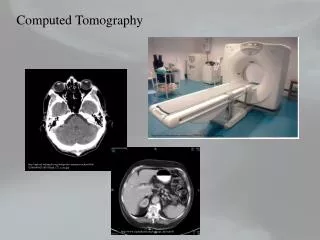
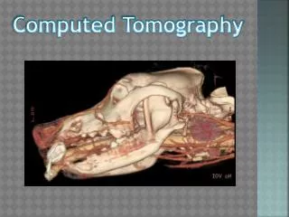
CT Imaging • Goal of x-ray CT is to reconstruct an image whose signal intensity at every point in region imaged is proportional to μ(x, y, z), where μ is linear attenuation coefficient for x-rays. • In practice, μis a function of x-ray energy as well as position and this introduces a number of complications that we will not investigate here. • X-ray CT is now a mature (though still rapidly developing) technology and a vital component of hospital diagnosis.
X-rays CT - 1st Generation • Single X-ray Pencil Beam • Single (1-D) Detector set at 180 degrees opposed • Simplest &cheapest scanner type but very slow due to • Translate(160 steps) • Rotate (1 degree) • ~ 5minutes (EMI CT1000) • Higher dose than fan-beam scanners • Scanners required head to be surrounded by water bag
Fig 1: Schematic diagram of a 1st generation CT scanner • (a) X-ray source projects a thin “pencil” beam of x-rays through sample, detected on the other side of the sample. Source and detector move in tandem along a gantry. (b) Whole gantry rotates, allowing projection data to be acquired at different angles.
Further generations of CT scanner • The first-generation scanner described earlier is capable of producing high-quality images. However, since the x-ray beam must be translated across the sample for each projection, the method is intrinsically slow. • Many refinements have been made over the years, the main function of which is to dramaticallyincrease the speed of data acquisition.
Further generations of CT scanner (cont’d) • Scanner using different types of radiation (e.g., fan beam) and different detection (e.g., many parallel strips of detectors) are known as different generations of X-ray CT scanner. We will not go into details here but provide only an overview of the key developments.
X-rays CT - 2nd Generation (~1980) • Narrow Fan Beam X-Ray • Small area (2-D) detector • Fan beam does not cover full body, so limited translation still required • Fan beam increases rotation step to ~10 degrees • Faster (~20 secs/slice) and lower dose • Stability ensured by each detector seeing non-attenuated x-ray beam during scan
X-rays CT - 3rd Generation • Wide-Angle Fan-Beam X-Ray • Large area (2-D) detector • Rotation Only - beam covers entire scan area • Even faster (~5 sec/slice) and even lower dose • Need very stable detectors, as some detectors are always attenuated • Xenon gas detectors offer best stability (and are inherently focussed, reducing scatter) • Solid State Detectors are more sensitive - can lead to dose savings of up to 40% - but at the risk of ring artefacts
X-rays CT – 3rd Generation Multi Slice Latest Developments - Spiral, multislice CT Cardiac CT
X-rays CT - 4th Generation (~1990) • Wide-Angle Fan-Beam X-Ray: Rotation Only • Complete 360 degree detector ring (Solid State - non-focussed, so scatter is removed post-acquisition mathematically) • Even faster (~1 sec/slice) and even lower dose • Not widely used – difficult to stabilise rotation + expensive detector • Fastest scanner employs electron beam, fired at ring of anode targets around patient to generate x-rays. • Slice acquired in ~10ms - excellent for cardiac work X-rays CT - Electron Beam 4th Generation
CT Scanner Construction: Gantry, Slip Ring, and Patient Table
Reconstruction of CT Images: Image Formation REFERENCE DETECTOR REFERENCE DETECTOR ADC PREPROCESSOR COMPUTER RAW DATA PROCESSORS BACK PROJECTOR CONVOLVED DATA RECONSTRUCTED DATA DISK TAPE DAC CRT DISPLAY
TheRadon transformation • In a first-generation scanner, the source-detector track can rotate around the sample, as shown in Fig 1. We will denote the “x-axis” along which the assembly slides when the assembly is at angle φ by xφ and the perpendicular axis by yφ. • Clearly, we may relate our (xφ,yφ) coordinates to the coordinates in the un-rotated lab frame by [5]
Figure 2: Relationship between Real Space and Radon Space Highlighted point on right shows where the value λφ(xφ) created by passing the x-ray beam through the sample at angle φ and point xφ is placed. Note that, as is conventional, the range of φ is [-π/ 2, +π / 2], since the remaining values of φ simply duplicate this range in the ideal case.
Hence, the “projection signal” when the gantry is at angle φ is [6] • We define the Radon transform as [7]
Radon Space • We define a new “space”, called Radon space, in much the same way as one defines reciprocal domains in a 2-D Fourier transform. Radon space has two dimensions xφ and φ . At the general point (xφ, φ), we “store” the result of the projection λφ(xφ). • Taking lots of projections at a complete range of xφ and φ “fills” Radon space with data, in much the same way that we filled Fourier space with our 2-D MRI data.
CT ‘X’ Axis ‘X’ Axis
CT ‘Y’ Axis ‘Y’ Axis
CT ‘Z’ Axis ‘Z’ Axis
CT Isocenter ISOCENTER
Fig 3. Sinograms for sample consisting of a small number of isolated objects. In this diagram, the full range of φ is [-π, +π] is displayed.
Relationship between “real space” and Radon space • Consider how the sinogram for a sample consisting of a single point in real (image) space will manifest in Radon space. • For a given angle φ, all locations xφ lead to λφ(xφ) = 0, except the one coinciding with the projection that goes through point (x0, y0) in real space. From Equation 5, this will be the projection where xφ = x0 cos φ + y0 sin φ.
Thus, all points in the Radon space corresponding to the single-point object are zero, except along the track [8] where R = (x2 + y2)1/2 and φ0 = tan-1 ( y / x). • If we have a composite object, then the filled Radon space is simply the sum of all the individual points making up the object (i.e. multiple sinusoids, with different values of R and φ0). See Fig 3 for an illustration of this.
Reconstruction of CT images (cont’d) • This is performed by a process known as back-projection, for which the procedure is as follows: • Consider one row of the sinogram, corresponding to angle φ. Note how in Fig 3, the value of the Radon transform λφ(xφ) is represented by the grey level of the pixel. When we look at a single row (i.e., a 1-D set of data), we can draw this as a graph — see Fig 4(a). Fig 4(b) shows a typical set of such line profiles at different projection angles.
Fig 4a. Relationship of 1-D projection through the sample and row in sinogram
Fig 4b. Projections at different angles correspond to different rows of the sinogram
Fig 4c. Back-projection of sinogram rows to form an image. The high-intensity areas of image correspond to crossing points of all three back-projections of profiles.
General Principles of Image Reconstruction • Image Display - Pixels and voxels
PIXEL Size Dependencies: • MATRIX SIZE • FOV
PIXEL vs VOXEL PIXEL VOXEL