Stereo Class - Chapter 7: Matching and Optimization
This chapter discusses the techniques of stereo matching, including standard stereo geometry, aggregation, optimization, and challenges faced in stereo vision. The Tsukuba dataset and the Geometric Computer Vision course schedule are also mentioned.


Stereo Class - Chapter 7: Matching and Optimization
E N D
Presentation Transcript
Stereo Class 7 Read Chapter 7 of tutorial http://cat.middlebury.edu/stereo/ Tsukuba dataset
Stereo • Standard stereo geometry • Stereo matching • Aggregation • Optimization (1D, 2D) • General camera configuration • Rectifications • Plane-sweep • Multi-view stereo
Challenges • Ill-posed inverse problem • Recover 3-D structure from 2-D information • Difficulties • Uniform regions • Half-occluded pixels
Pixel Dissimilarity • Absolute difference of intensities c=|I1(x,y)- I2(x-d,y)| • Interval matching [Birchfield 98] • Considers sensor integration • Represents pixels as intervals
Alternative Dissimilarity Measures • Rank and Census transforms [Zabih ECCV94] • Rank transform: • Define window containing R pixels around each pixel • Count the number of pixels with lower intensities than center pixel in the window • Replace intensity with rank (0..R-1) • Compute SAD on rank-transformed images • Census transform: • Use bit string, defined by neighbors, instead of scalar rank • Robust against illumination changes
Rank and Census Transform Results • Noise free, random dot stereograms • Different gain and bias
Systematic Errors of Area-based Stereo • Ambiguous matches in textureless regions • Surface over-extension [Okutomi IJCV02]
Surface Over-extension • Expected value of E[(x-y)2] for x in left and y in right image is: Case A: σF2+ σB2+(μF- μB)2 for w/2-λ pixels in each row Case B: 2 σB2 for w/2+λ pixels in each row Left image Disparity of back surface Right image
Surface Over-extension • Discontinuity perpendicular to epipolar lines • Discontinuity parallel to epipolar lines Left image Disparity of back surface Right image
Over-extension and shrinkage • Turns out that: for discontinuities perpendicular to epipolar lines • And:for discontinuities parallel to epipolar lines
Equivalent to using minnearby cost • Result: loss of depth accuracy Offset Windows
Discontinuity Detection • Use offset windows only where appropriate • Bi-modal distribution of SSD • Pixel of interest different than mode within window
Compact Windows • [Veksler CVPR03]: Adapt windows size based on: • Average matching error per pixel • Variance of matching error • Window size (to bias towards larger windows) • Pick window that minimizes cost
A C B D Shaded area = A+D-B-CIndependent of size Integral Image Sum of shaded part Compute an integral image for pixel dissimilarity at each possible disparity
Rod-shaped filters • Instead of square windows aggregate cost in rod-shaped shiftable windows [Kim CVPR05] • Search for one that minimizes the cost (assume that it is an iso-disparity curve) • Typically use 36 orientations
Locally Adaptive Support Apply weights to contributions of neighboringpixels according to similarity and proximity [Yoon CVPR05]
Locally Adaptive Support • Similarity in CIE Lab color space: • Proximity: Euclidean distance • Weights:
Locally Adaptive Support: Results Locally Adaptive Support
Occlusions (Slide from Pascal Fua)
Ordering constraint surface slice surface as a path 6 5 occlusion left 4 3 2 1 4,5 6 1 2,3 5 6 2,3 4 occlusion right 1 3 6 1 2 4,5
Uniqueness constraint • In an image pair each pixel has at most one corresponding pixel • In general one corresponding pixel • In case of occlusion there is none
use reconstructed features to determine bounding box Disparity constraint surface slice surface as a path bounding box disparity band constant disparity surfaces
Similarity measure (SSD or NCC) Optimal path (dynamic programming ) Stereo matching • Constraints • epipolar • ordering • uniqueness • disparity limit • Trade-off • Matching cost (data) • Discontinuities (prior) Consider all paths that satisfy the constraints pick best using dynamic programming
Hierarchical stereo matching Allows faster computation Deals with large disparity ranges Downsampling (Gaussian pyramid) Disparity propagation
Disparity map image I´(x´,y´) image I(x,y) Disparity map D(x,y) (x´,y´)=(x+D(x,y),y)
Semi-global optimization • Optimize: E=Edata+E(|Dp-Dq|=1)+E(|Dp-Dq|>1) [Hirshmüller CVPR05] • Use mutual information as cost • NP-hard using graph cuts or belief propagation (2-D optimization) • Instead do dynamic programming along many directions • Don’t use visibility or ordering constraints • Enforce uniqueness • Add costs
Results of Semi-global optimization No. 1 overall in Middlebury evaluation(at 0.5 error threshold as of Sep. 2006)
Energy minimization (Slide from Pascal Fua)
Graph Cut (general formulation requires multi-way cut!) (Slide from Pascal Fua)
Simplified graph cut (Roy and Cox ICCV‘98) (Boykov et al ICCV‘99)
Belief Propagation Belief of one node about another gets propagated through messages (full pdf, not just most likely state) first iteration per pixel +left +up +right +down subsequent iterations 4 ... 5 3 20 2 (adapted from J. Coughlan slides)
~ image size (calibrated) Planar rectification Distortion minimization (uncalibrated) Bring two views to standard stereo setup (moves epipole to ) (not possible when in/close to image)
Polar rectification (Pollefeys et al. ICCV’99) Polar re-parameterization around epipoles Requires only (oriented) epipolar geometry Preserve length of epipolar lines Choose so that no pixels are compressed original image rectified image Works for all relative motions Guarantees minimal image size
original image pair planar rectification polar rectification
Example: Béguinage of Leuven Does not work with standard Homography-based approaches