Advanced Stereo Techniques in Photography: A Comprehensive Guide
This comprehensive guide delves into advanced stereo techniques, such as epipolar geometry, depth estimation, rectification, and calibration, to enhance your photographic skills. Learn about stereo panoramas, matching algorithms, and the principles of triangulation. Explore the history of stereo photography and discover valuable resources and tools for improving your stereo imaging projects.


Advanced Stereo Techniques in Photography: A Comprehensive Guide
E N D
Presentation Transcript
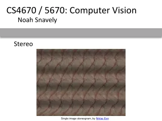
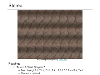
Stereo • Binocular Stereo • Motivation • Epipolar geometry • Matching • Depth estimation • Rectification • Calibration (finish up) • Next Time • Multiview stereo
Public Library, Stereoscopic Looking Room, Chicago, by Phillips, 1923
Mark Twain at Pool Table", no date, UCR Museum of Photography
Woman getting eye exam during immigration procedure at Ellis Island, c. 1905 - 1920, UCR Museum of Phography
Stereograms online • UCR stereographs • http://www.cmp.ucr.edu/site/exhibitions/stereo/ • The Art of Stereo Photography • http://www.photostuff.co.uk/stereo.htm • History of Stereo Photography • http://www.rpi.edu/~ruiz/stereo_history/text/historystereog.html • Double Exposure • http://home.centurytel.net/s3dcor/index.html • Stereo Photography • http://www.shortcourses.com/book01/chapter09.htm • 3D Photography links • http://www.studyweb.com/links/5243.html • National Stereoscopic Association • http://204.248.144.203/3dLibrary/welcome.html • Books on Stereo Photography • http://userwww.sfsu.edu/~hl/3d.biblio.html
[Ishiguro, Yamamoto, Tsuji 92] • [Peleg and Ben-Ezra 99] • [Shum, Kalai, Seitz 99] Stereo Panoramas • Interactive demo: http://www.cs.columbia.edu/CAVE/
Disparity map result Depth from Stereo Panoramas
Stereo scene point image plane optical center
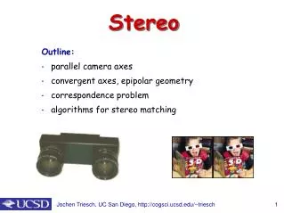
Stereo • Basic Principle: Triangulation • Gives reconstruction as intersection of two rays • Requires • calibration • point correspondence
epipolar line epipolar line epipolar plane Stereo Correspondence • Determine Pixel Correspondence • Pairs of points that correspond to same scene point • Epipolar Constraint • Reduces correspondence problem to 1D search along conjugateepipolar lines • Java demo: http://www.ai.sri.com/~luong/research/Meta3DViewer/EpipolarGeo.html
Epipolar Geometry • All camera rays lie in a “pencil” of planes
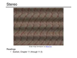
Stereo Matching • Features vs. Pixels? • Do we extract features prior to matching? Julesz-style Random Dot Stereogram
Stereo Matching Algorithms • Match Pixels in Conjugate Epipolar Lines • Assume color of point does not change • Pitfalls • specularities • low-contrast regions • occlusions • image error • camera calibration error • Numerous approaches • dynamic programming [Baker 81,Ohta 85] • smoothness functionals • more images (trinocular, N-ocular) [Okutomi 93] • graph cuts [Boykov 00]
For each epipolar line For each pixel in the left image Improvement: match windows Your Basic Stereo Algorithm • compare with every pixel on same epipolar line in right image • pick pixel with minimum match cost
Window Size • Smaller window • more details • more noise • Larger window • less noise • less detail W = 3 W = 20 • Better results with adaptive window • T. Kanade and M. Okutomi,A Stereo Matching Algorithm with an Adaptive Window: Theory and Experiment,, Proc. International Conference on Robotics and Automation, 1991. • D. Scharstein and R. Szeliski. Stereo matching with nonlinear diffusion. International Journal of Computer Vision, 28(2):155-174, July 1998
Stereo as Energy Minimization • Matching Cost Formulated as Energy • “data” term penalizing bad matches • “neighborhood term” encouraging spatial smoothness
edge weight d3 d2 d1 edge weight Stereo as a Graph Problem [Boykov, 1999] • Pixels Labels (disparities)
d3 d2 d1 Stereo as a Graph Problem [Boykov, 1999] • Graph Cost • Matching cost between images • Meighborhood matching term • Goal: figure out which labels are connected to which pixels
d3 d2 d1 Stereo Matching by Graph Cuts • Graph Cut • Delete enough edges so that • each pixel is (transitively) connected to exactly one label node • Cost of a cut: sum of deleted edge weights • Finding min cost cut equivalent to finding global minimum of energy function
Computing a multiway cut • With 2 labels: classical min-cut problem • Solvable by standard flow algorithms • polynomial time in theory, nearly linear in practice • More than 2 terminals: NP-hard [Dahlhaus et al., STOC ‘92] • Efficient approximation algorithms exist • Within a factor of 2 of optimal • Computes local minimum in a strong sense • even very large moves will not improve the energy • Yuri Boykov, Olga Veksler and Ramin Zabih, Fast Approximate Energy Minimization via Graph Cuts, International Conference on Computer Vision, September 1999.
Red-blue swap move Green expansion move Move Examples Starting point
B A AB subgraph (run min-cut on this graph) The Swap Move Algorithm 1. Start with an arbitrary labeling 2. Cycle through every label pair (A,B) in some order 2.1 Find the lowest E labeling within a single AB-swap 2.2 Go there if it’s lower E than the current labeling 3. If E did not decrease in the cycle, we’re done Otherwise, go to step 2 B A Original graph
The expansion move algorithm 1. Start with an arbitrary labeling 2. Cycle through every label A in some order 2.1 Find the lowest E labeling within a single A-expansion 2.2 Go there if it’s lower E than the current labeling 3. If E did not decrease in the cycle, we’re done Otherwise, go to step 2
Stereo Results • Data from University of Tsukuba • Similar results on other images without ground truth Scene Ground truth
Results with Window Correlation Normalized correlation (best window size) Ground truth
Results with Graph Cuts Graph Cuts (Potts model E, expansion move algorithm) Ground truth
depth map 3D rendering [Szeliski & Kang ‘95] X z u u’ f f baseline C C’ Depth from Disparity input image (1 of 2)
Disparity-Based Rendering • Render new views from raw disparity • S. M. Seitz and C. R. Dyer, View Morphing, Proc. SIGGRAPH 96, 1996, pp. 21-30. • L. McMillan and G. Bishop. Plenoptic Modeling: An Image-Based Rendering System, Proc. of SIGGRAPH 95, 1995, pp. 39-46.
Image Rectification • Image Reprojection • reproject image planes onto common plane parallel to line between optical centers • a homography (3x3 transform)applied to both input images • C. Loop and Z. Zhang. Computing Rectifying Homographies for Stereo Vision. IEEE Conf. Computer Vision and Pattern Recognition, 1999.
Stereo Reconstruction Pipeline • Steps • Calibrate cameras • Rectify images • Compute disparity • Estimate depth
H depends on camera parameters (A, R, t) where Calibration from (unknown) Planes • What’s the image of a plane under perspective? • a homography (3x3 projective transformation) • preserves lines, incidence, conics • Given 3 homographies, can compute A, R, t • Z. Zhang. A flexible new technique for camera calibration. IEEE Transactions on Pattern Analysis and Machine Intelligence, 22(11):1330-1334, 2000. • http://research.microsoft.com/~zhang/Calib/
3. Introduce radial distortion model • Solve for A, R, t, k1, k2 • nonlinear optimization (using Levenberg-Marquardt) Calibration from Planes • 1. Compute homography Hi for 3+ planes • Doesn’t require knowing 3D • Does require mapping between at least 4 points on plane and in image (both expressed in 2D plane coordinates) • 2. Solve for A, R, t from H1, H2, H3 • 1plane if only f unknown • 2 planes if (f,uc,vc) unknown • 3+ planes for full K