Stereo
Stereo. Outline: parallel camera axes convergent axes, epipolar geometry correspondence problem algorithms for stereo matching. Credits: major sources of material, including figures and slides were: Forsyth, D.A. and Ponce, J., Computer Vision: A Modern Approach, Prentice Hall, 2003

Stereo
E N D
Presentation Transcript
Stereo • Outline: • parallel camera axes • convergent axes, epipolar geometry • correspondence problem • algorithms for stereo matching
Credits: major sources of material, including figures and slides were: • Forsyth, D.A. and Ponce, J., Computer Vision: A Modern Approach, Prentice Hall, 2003 • Mallot, H.-P., Computational Vision • Slides: Octavia Camps, Frank Dellaert, Davi Geiger, David Jacobs, Jim Rehg, Steve Seitz, Zhigang Zhu • and various resources on the WWW
depth baseline Overview Triangulate on two images of the same point to recover depth. • Feature matching across views • Calibrated cameras Left Right Matching correlation windows across scan lines
Virtual Image Pinhole Camera Model Image plane Focal length f Center of projection
Pinhole Camera Model Image plane Virtual Image
Basic Stereo Derivations disparity
Stereo with Converging Cameras • Stereo with Parallel Axes • Short baseline • large common FOV • large depth error • Long baseline • small depth error • small common FOV • More occlusion problems • Two optical axes intersect at the Fixation Point • converging angle q • The common FOV Increases FOV Left right
FOV Left right Stereo with Converging Cameras • Stereo with Parallel Axes • Short baseline • large common FOV • large depth error • Long baseline • small depth error • small common FOV • More occlusion problems • Two optical axes intersect at the Fixation Point • converging angle q • The common FOV Increases
Stereo with Converging Cameras • Two optical axes intersect at the Fixation Point • converging angle q (vergence) • The common FOV Increases • Disparity properties • Disparity uses angle instead of distance • Zero disparity at fixation point • and the Zero-disparity horopter • Disparity increases with the distance of objects from the fixation points • >0 : outside of the horopter • <0 : inside the horopter • Depth Accuracy vs. Depth • Depth Error Depth2 • Nearer the point, better the depth estimation Fixation point FOV q Left right
Stereo with Converging Cameras • Two optical axes intersect at the Fixation Point • converging angle q • The common FOV Increases • Disparity properties • Disparity uses angle instead of distance • Zero disparity at fixation point • and the Zero-disparity horopter • Disparity increases with the distance of objects from the fixation points • >0 : outside of the horopter • <0 : inside the horopter • Depth Accuracy vs. Depth • Depth Error Depth2 • Nearer the point, better the depth estimation Fixation point Horopter q al ar ar = al da = 0 Left right
Stereo with Converging Cameras • Two optical axes intersect at the Fixation Point • converging angle q • The common FOV Increases • Disparity properties • Disparity uses angle instead of distance • Zero disparity at fixation point • and the Zero-disparity horopter • Disparity increases with the distance of objects from the fixation points • >0 : outside of the horopter • <0 : inside the horopter • Depth Accuracy vs. Depth • Depth Error Depth2 • Nearer the point, better the depth estimation Fixation point Horopter q al ar ar > al da > 0 Left right
Stereo with Converging Cameras • Two optical axes intersect at the Fixation Point • converging angle q • The common FOV Increases • Disparity properties • Disparity uses angle instead of distance • Zero disparity at fixation point • and the Zero-disparity horopter • Disparity increases with the distance of objects from the fixation points • >0 : outside of the horopter • <0 : inside the horopter • Depth Accuracy vs. Depth • Depth Error Depth2 • Nearer the point, better the depth estimation Fixation point Horopter ar aL ar < al da < 0 Left right
Stereo with Converging Cameras • Two optical axes intersect at the Fixation Point • converging angle q • The common FOV Increases • Disparity properties • Disparity uses angle instead of distance • Zero disparity at fixation point • and the Zero-disparity horopter • Disparity increases with the distance of objects from the fixation points • >0 : outside of the horopter • <0 : inside the horopter • Depth Accuracy vs. Depth • Depth Error Depth2 • Nearer the point, better the depth estimation Fixation point Horopter al ar D(da) ? Left right
P Pl Pr Yr p p r l Yl Xl Zl Zr fl fr Ol Or R, T Xr Parameters of a Stereo System • Intrinsic Parameters • Characterize the transformation from camera to pixel coordinate systems of each camera • Focal length, image center, aspect ratio • Extrinsic parameters • Describe the relative position and orientation of the two cameras • Rotation matrix R and translation vector T
P Pl Pr Epipolar Plane Epipolar Lines p p r l Ol el er Or Epipoles Epipolar Geometry • Motivation: where to search correspondences? • Epipolar Plane • A plane going through point P and the centers of projection (COPs) of the two cameras • Conjugated Epipolar Lines • Lines where epipolar plane intersects the image planes • Epipoles • The image in one camera of the COP of the other • Epipolar Constraint • Corresponding points must lie on conjugated epipolar lines
Epipolar geometry thanks to Andrew Zisserman and Richard Hartley for all figures.
Epipolar geometry • For any two fixed cameras we have one baseline. • For any 3d point X we have a different epipolar plane pi. • All epipolar planes intersect at the baseline.
Epipolar line • Suppose we know only x and the baseline. • How is the corresponding point x’ in the other image constrained? • pi is defined by the baseline and the ray Cx. • The epipolar line l’ is the image of this ray in the other image. x’ must lie on l’. • The benefit of the epipolar line is that the correspondence search can be restricted to l’ instead of searching the entire image.
epipolar line epipolar line epipolar plane The epipolar constraint • Epipolar Constraint • Matching points lie along corresponding epipolar lines • Reduces correspondence problem to 1D search along conjugateepipolar lines • Greatly reduces cost and ambiguity of matching Slide credit: Steve Seitz
Epipolar terminology • Epipole: • intersection of the line joining the camera centers (baseline) and the image plane. • the image of the other camera center in the image plane. • intersection of the epipolar lines. • Epipolar plane: • a plane containing the baseline. There is a one-parameter family of epipolar planes for a fixed camera pair. • Epipolar line: • intersection of the epipolar plane with the image plane. • all epipolar lines intersect in the epipole. • an epipolar plane intersects both image planes and defines correspondences between the lines.
P p p r l Ol Or Reconstruction by Triangulation • Assumption and Problem • Under the assumption that both intrinsic and extrinsic parameters are known • Compute the 3-D location from their projections, pl and pr • Solution • Triangulation: Two rays are known and the intersection can be computed • Problem: Two rays will not actually intersect in space due to errors in calibration and correspondences, and sampling • Solution: find a point in space with minimum distance from both rays
Simplest Case from above assume: • Image planes of cameras are parallel • Focal points are at same height • Focal lengths same then: • epipolar lines fall along the horizontal scan lines of the images
Rectification • Motivation: • create case from above since it: • simplifies algorithms • improves efficiency • Image Reprojection • reproject image planes onto common plane parallel to line between optical centers • Notice, only focal point of camera really matters (Seitz)
Correspondence • It is fundamentally ambiguous, even with stereo constraints: many 3D points could have given rise to the observed features
What should we match? • Objects? • Edges? • Pixels? • Collections of pixels? Visual illusions: • double nail illusion • line illusion
Human Stereo: Random Dot Stereogram Julesz’s Random Dot Stereogram. The left image, a black and white image, is generated by a program that assigns black or white values at each pixel according to a random number generator. The right image is constructed from by copying the left image, but an imaginary square inside the left image is displaced a few pixels to the left and the empty space filled with black and white values chosen at random. When the stereo pair is shown, the observers can identify/match the imaginary square on both images and consequently “see” a square in front of the background. It shows that stereo matching can occur without recognition.
Correspondence: Epipolar constraint. The epipolar constraint helps, but much ambiguity remains.
Correspondence: Photometric constraint • Same world point has same intensity in both images. • True for Lambertian fronto-parallel surfaces • Violations: • Noise • Specularity • Foreshortening
Correspondence: other constraints • ordering constraint: • uniqueness constraint: • every feature in one image has only one match in the other image • but: transparency
For each epipolar line For each pixel in the left image Improvement: match windows Pixel matching • compare with every pixel on same epipolar line in right image • pick pixel with minimum match cost • This leaves too much ambiguity, so: (Seitz)
Correspondence Using Correlation Left Right scanline SSD error disparity Left Right
Sum of Squared (Pixel) Differences Left Right
Image Normalization • Even when the cameras are identical models, there can be differences in gain and sensitivity. • For these reason and more, it is a good idea to normalize the pixels in each window:
Images as Vectors Left Right “Unwrap” image to form vector, using raster scan order row 1 row 2 Each window is a vectorin an m2 dimensionalvector space.Normalization makesthem unit length. row 3
Image Metrics (Normalized) Sum of Squared Differences Normalized Correlation
Stereo Results Images courtesy of Point Grey Research
W = 3 W = 20 Window size • Effect of window size • Some approaches have been developed to use an adaptive window size (try multiple sizes and select best match) (Seitz)
Stereo testing and comparisons D. Scharstein and R. Szeliski. "A Taxonomy and Evaluation of Dense Two-Frame Stereo Correspondence Algorithms," International Journal of Computer Vision,47 (2002), pp. 7-42. Scene Ground truth
Results with window correlation Window-based matching (best window size) Ground truth (Seitz)
Results with better method State of the art method: Graph cuts Ground truth (Seitz)
… … Stereo Correspondences Left scanline Right scanline
… … Match Match Match Occlusion Disocclusion Stereo Correspondences Left scanline Right scanline
Occluded Pixels Search Over Correspondences Three cases: • Sequential – add cost of match (small if intensities agree) • Occluded – add cost of no match (large cost) • Disoccluded – add cost of no match (large cost) Left scanline Right scanline Disoccluded Pixels
Occluded Pixels Stereo Matching with Dynamic Programming Dynamic programming yields the optimal path through grid. This is the best set of matches that satisfy the ordering constraint Left scanline Start Dis-occluded Pixels Right scanline End
Dynamic Programming • Efficient algorithm for solving sequential decision (optimal path) problems. 1 1 1 1 … 2 2 2 2 3 3 3 3 How many paths through this trellis?