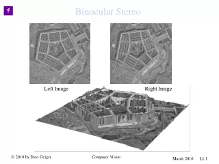
Binocular Stereo
Binocular Stereo. Philippos Mordohai University of North Carolina at Chapel Hill. September 21, 2006. Outline. Introduction Cost functions Challenges Cost aggregation Optimization Binocular stereo algorithms. Stereo Vision. Match something Feature-based algorithms

Binocular Stereo
E N D
Presentation Transcript
Binocular Stereo Philippos Mordohai University of North Carolina at Chapel Hill September 21, 2006
Outline • Introduction • Cost functions • Challenges • Cost aggregation • Optimization • Binocular stereo algorithms
Stereo Vision • Match something • Feature-based algorithms • Area-based algorithms • Apply constraints to help convergence • Smoothness/Regularization • Ordering • Uniqueness • Visibility • Optimize something (typically) • Need energy/objective function that can be optimized
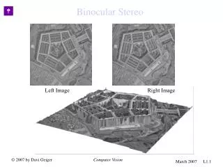
Binocular Datasets Middlebury data (www.middlebury.edu/stereo)
Challenges • Ill-posed inverse problem • Recover 3-D structure from 2-D information • Difficulties • Uniform regions • Half-occluded pixels
Pixel Dissimilarity • Absolute difference of intensities • c=|I1(x,y)- I2(x-d,y)| • Interval matching [Birchfield 98] • Considers sensor integration • Represents pixels as intervals
Alternative Dissimilarity Measures • Rank and Census transforms [Zabih ECCV94] • Rank transform: • Define window containing R pixels around each pixel • Count the number of pixels with lower intensities than center pixel in the window • Replace intensity with rank (0..R-1) • Compute SAD on rank-transformed images • Census transform: • Use bit string, defined by neighbors, instead of scalar rank • Robust against illumination changes
Rank and Census Transform Results • Noise free, random dot stereograms • Different gain and bias
Outline • Introduction • Cost functions • Challenges • Cost aggregation • Optimization • Binocular stereo algorithms
Systematic Errors of Area-based Stereo • Ambiguous matches in textureless regions • Surface over-extension [Okutomi IJCV02]
Surface Over-extension • Expected value of E[(x-y)2] for x in left and y in right image is: • Case A: σF2+ σB2+(μF- μB)2 for w/2-λ pixels in each row • Case B: 2 σB2 for w/2+λ pixels in each row Left image Disparity of back surface Right image
Surface Over-extension • Discontinuity perpendicular to epipolar lines • Discontinuity parallel to epipolar lines Left image Disparity of back surface Right image
Over-extension and shrinkage • Turns out that: for discontinuities perpendicular to epipolar lines • And:for discontinuities parallel to epipolar lines
Equivalent to using minnearby cost • Result: loss of depth accuracy Offset Windows
Discontinuity Detection • Use offset windows only where appropriate • Bi-modal distribution of SSD • Pixel of interest different than mode within window
Outline • Introduction • Cost functions • Challenges • Cost aggregation • Optimization • Binocular stereo algorithms
Compact Windows • [Veksler CVPR03]: Adapt windows size based on: • Average matching error per pixel • Variance of matching error • Window size (to bias towards larger windows) • Pick window that minimizes cost
A C B D Shaded area = A+D-B-CIndependent of size Integral Image Sum of shaded part Compute an integral image for pixel dissimilarity at each possible disparity
Rod-shaped filters • Instead of square windows aggregate cost in rod-shaped shiftable windows [Kim CVPR05] • Search for one that minimizes the cost (assume that it is an iso-disparity curve) • Typically use 36 orientations
Locally Adaptive Support Apply weights to contributions of neighboringpixels according to similarity and proximity [Yoon CVPR05]
Locally Adaptive Support • Similarity in CIE Lab color space: • Proximity: Euclidean distance • Weights:
Outline • Introduction • Cost functions • Challenges • Cost aggregation • Optimization • Binocular stereo algorithms
Constraints • Results of un-sophisticated local operators still noisy • Optimization required • Need constraints • Smoothness • Ordering • Uniqueness • Visibility • Energy function:
Ordering Constraint • If A is on the left of B in reference image => the match for A has to be on the left of the match of B in target image • Violated by thin objects • But, useful for dynamic programming Image from Sun et al. CVPR05
Left image Right image Right occlusion p p+ d p correspondence p Left occlusion t s q Dynamic Programming
Dynamic Programming without the Ordering Constraint • Two Pass Dynamic Programming [Kim CVPR05] • Use reliable matches found with rod-shaped filters as “ground control points” • No ordering • Second pass along columns to enforce inter-scanline consistency
Dynamic Programming without the Ordering Constraint • Use GPU [Gong CVPR05] • Calculate 3-D matrix (x,y,d) of matching costs • Aggregate using shiftable 3x3 window • Find reliable matches along horizontal lines • Find reliable matches along vertical lines • Fill in holes • Match reliability = cost of scanline passing through match – cost of scanline not passing through match
Near Real-time Results 10-25 frames per second depending on image size and disparity range
Semi-global optimization • Optimize: E=Edata+E(|Dp-Dq|=1)+E(|Dp-Dq|>1) [Hirshmüller CVPR05] • Use mutual information as cost • NP-hard using graph cuts or belief propagation (2-D optimization) • Instead do dynamic programming along many directions • Don’t use visibility or ordering constraints • Enforce uniqueness • Add costs
Results of Semi-global optimization No. 1 overall in Middlebury evaluation(at 0.5 error threshold as of Sep. 2006)
cut t labels “cut” L(p) Disparity labels y y s p x x 2-D Optimization • Energy: Data Term + Regularization • Find minimum cost cut that separates source and target
labels labels “cut” L(p) L(p) y p x x p Scanline vs.Multi-scanline optimization s-t Graph Cuts (multi-scan-line optimization) Dynamic Programming (single scan line optimization)
V D D V V D D V Graph-cuts • MRF Formulation • In general suffers from multiple local minima • Combinatorial optimization: minimize costiSDi(fi) + (i,j)N V(fi,fj) over discrete space of possible labelings f • Exponential search space O(kn) • NP hard in most cases for grid graph • Approximate practical solution [Boykov PAMI01]
Red expansion move from f Alpha Expansion Technique • Use min-cut to efficiently solve a special two label problem • Labels “stay the same” or “replace with a” • Iterate over possible values of a • Each rules out exponentially many labelings Input labeling f
Results using Graph-Cuts • Include occlusion term in energy [Kolmogorov ICCV01]
D V V D D D V V D Belief Propagation • Local message passing scheme in graph • Every site (pixel) in parallel computes a belief • pdf of local estimatesof label costs • Observation: data term (fixed) • Messages: pdf’s from node to neighbors • Exact solution for trees, good approximation for graphs with cycles
Belief Propagation for Stereo • Minimize energy that considers matching cost, depth discontinuities and occlusion [Sun ECCV02, PAMI03]
Uniqueness Constraint • Each pixel can have exactly one or no match in the other image • Used in most of the above methods • Unfortunately, surfaces do not project to the same number of pixels in both images [Ogale CVPR04]
Continuous Approach • Treat intervals on scanlines as continuous entities and not as discrete sets of pixels • Assign disparity to beginning and end of each interval • Optimize each scanline • Would rank 8,7 and 2 for images without horizontal slant • Ranks 22 for Venus !!!
Visibility Constraint • Each pixel is either occluded or can have one disparity value (possibly subpixel) associated with it [Sun CVPR05] • Allows for many-to-one correspondence • Symmetric treatment of images • Compute both disparity and occlusion maps • Left occlusion derived from right disparity and right occlusion from left disparity • Optimize using Belief Propagation • Iterate between disparity and occlusion maps • Segmentation as a soft constraint
Results using Symmetric Belief Propagation No. 3 in Middlebury evaluation (No. 1 in New Middlebury evaluation) (June 2005) No. 1 in Middlebury evaluation (June 2005)
Results using Symmetric Belief Propagation No. 1 in Middlebury evaluation(June 2005) No. 1 in Middlebury evaluation(June 2005)