Binocular Stereo
Binocular Stereo. Topics. Principle basic equation epipolar line features and strategies for matching Case study Block matching Relaxation DP stereo. Basic principles. single image is ambiguous. A. a”. a’. another image taken from a different direction gives the unique 3D point.

Binocular Stereo
E N D
Presentation Transcript
Topics • Principle • basic equation • epipolar line • features and strategies for matching • Case study • Block matching • Relaxation • DP stereo
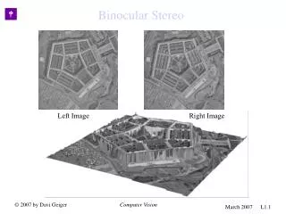
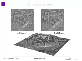
single image is ambiguous A a” a’ another image taken from a different direction gives the unique 3D point Binocular stereo
Base line Epipolar line One image point Possible line of sight Epipolar plane Epipolar line constraints Corresponding points lie on the Epipolar lines Epipolar line constratints
C2 C1 Epipoles • intersections of baseline with image planes • projection of the optical center in another image • the vanishing points of camera motion direction e2 e1
rectification Rectification
Terminology A physical point left image point right image point right image plane left image plane focal length right image center z left image center World coordinate system base line length
v u (X, Y, Z) (u, v) Image plane Y X -Z Perspective Projection View point (Optical center) f : focal length
d + x d - x Basic binocular stereo equation z=-2df/(x”-x’) x”-x’: disparity 2d : base line length -z x’ x” f d d z
Features for matching 10 11 12 10 11 12 10 11 12 10 11 12 11 15 16 a. brightness b. edges c. edge intervals d. interest points
Strategies for matching 10 10 10 10 5 10 10 10 10 10 10 10 10 5 10 10 10 10 10 10 10 10 10 10 10 10 10 a. relaxation b. coarse to fine c. dynamic programming global optimam local optimam local optimam
Classification of stereo methods • Features for matching • brightness value • point • edge • region • Strategies for matching • brute-force • coarse-to-fine • relaxation • dynamic programming • Constraints for matching • epipolar lines • disparity limit • continuity • uniqueness
Block-Matching Stereo 1. method b c • 2. problem • a. trade-off of window size and resolution • b. dull peak b c b c
Cost Function d Near Object Near Object Background Background right left (a) SAD (sum. of absolute difference) (b) SSD (sum. of squared difference) (c) Correlation
Moravec Stereo(`79) navigation Moravec “Visual mapping by a robot rover” Proc 6th IJCAI,pp.598-600 (1979)
Moravec’s cart Slide stereo Motion stereo
Slider stereo (9 eyes stereo) • 9C2 = 36 stereo pairs!!! • each stereo has an uncertainty measure • uncertainty = 1 / base-line • each stereo has a confidence measure long base line large uncertainty
matching expand matching expand matching Coarse to fine
area:confidence measure σ estimated distance σ:uncertainty measure Interest point 9C2 = 36 curves
Moravec Stereo(`81) • 1. Features for matching • a. brightness value • b. point • c. edge • d. region • 2. Strategies for matching • a. brute-force (not a strategy ???) • b. coarse-to-fine • c. relaxation • d. dynamic programming • 3. Constraints for matching • a. epipolar lines • b. disparity limit • c. continuity • d. Uniqueness • Purpose: navigation (Stanford) interest point
Recent Progress disparity Near Object Near Object Background Background right left How to estimate the disparities? Minimize some cost function along the epipolar line disparity H. Hirschnuller, "Improvements in Real-Time Correlation-Based Stereo Vision", IEEE Workshop on Stereo and Multi-Baseline Vision, 2001
Fatting Effect on Object Boundary • No single window fits at the discontinuity ⇒ Fatting effect of the object Foreground Correspondence Near Object Near Object Background Background Background Correspondence right left
Accurate Estimation on Object Boundary • Shiftable Window d c1 c1 c2 c0 c0 c3 c3 c4 Near Object Near Object are used. Background Background right left Min{c1,c2,c3,c4} Min{{c1,c2,c3,c4}-c’} disparity
1st search 2nd search Consistency Checking • Check if two independent disparity estimation coincide • Left ⇒Right search • Right ⇒Left search • Inconsistent disparities are considered as a false match Epipolar line Epipolar line Check if they coincide left right
Result • SAD with 11x11 window • Shiftable window + consistency checking Left image Disparity map
Cooperative stereo:Marr-Poggio Stereo(`76) Simulating human visual system (random dot stereo gram) Marr,Poggio “Cooperative computation of stereo disparity” Science 194,283-287
Input : random dot stereo left image random dot shift the catch pat right image we can see the height different between the central and peripheral area
Constraints • Epipolar line constraint • Uniqueness constraint • each point in a image has only one depth value O.K.No. • Continuity constraint • each point is almost sure to have a depth value near the values of neighbors O.K. No.
D E F A B C A B D E F C Uniqueness constraint prohibits two or more matching points on one horizontal or vertical lines continuity constraint attracts more matching on a diagonal line (E-A) A B C (E-B) prohibit (E-C) (D-A) attract (E-B) Same depth (F-C) attract
Relaxation 10 10 10 10 5 10 10 10 10 10 10 10 10 5 10 10 10 10 10 10 10 10 10 10 10 10 10 n n+1
Marr-Poggio Stereo (`76) • 1. Features for matching • a. brightness value • b. point • c. edge • d. region • 2. Strategies for matching • a. brute-force • b. coarse-to-fine • c. relaxation • d. dynamic programming • 3. Constraints for matching • a. epipolar lines • b. disparity limit • c. continuity • d. uniqueness • Purpose: simulate the human visual system (MIT)
Recent progress:Graph-cut • Solve graph partition problem in globally optimal way • Formulate the problem in energy minimization framework • Design a graph such that the sum of cut edges equals to the total energy • Find a “Cut” that minimizes the energy Cut i j Vij
Example of Graph-cut • Image segmentation Graph partition Segmentation Graph={N,e} Ni: Graph node eij: Edge connecting nodes C: Cut Image={pixel} Vij: Similarity between neighboring pixels Foreground/Background boundary Nj Ni Vij
Solution to a Graph-cut Problem • Min-Cut/Max-Flow algorithm • Given source (s) and sink nodes (t) • Define capacity on each edge • Find the maximum flow from s⇒t, satisfying capacity constraints, and cut the bottleneck Flow i Source Sink j Bottleneck Min-Cut = Max-Flow Yuri Boykov, Vladimir Kolmogorov, "An Experimental Comparison of Min-Cut/Max-Flow Algorithms for Energy Minimization in Vision", PAMI, 2004
Multi-label Problem • Find the labeling f that minimizes the energy measures the extent to which f is not piece wise smooth measures the disagreement between f and the observed data Measures how well label fp fits pixel p given the observed data Smoothness penalty between adjacent (N) pixels Yuri Boykov and Olga Veksler and Ramin Zabih, “Fast Approximate Energy Minimization via Graph Cuts,” ICCV, 2001
Multi-label Solution via Graph-cut • Iterative graph-cut approach • 2 types of move algorithm are proposed • αβ-swap • α-expansion Minimize E under cond. is preserved γ β Graph-cut α Minimize E under cond. can be changed to α γ β Graph-cut α
αβ-swap Algorithm • Start with an arbitrary labeling f • Success:= 0 • For each pair of labels • Find f’=arg min E(f’) among f’ within one αβ-swap of f • If E(f’) < E(f) then f’:=f and success:=1 • If success=1 goto 2 • Return f γ β α
αβ-swap Graph Structure edge weight for α p q r s should be a semi metric β
αβ-swap Cut • 3 possible cases α α α Cut p q p q p q α α β β β α Cut Cut β β β
α-expansion Algorithm • Start with an arbitrary labeling f • Success:= 0 • For each label • Find f’=arg min E(f’) among f’ within one α-expansion of f • If E(f’) < E(f) then f’:=f and success:=1 • If success=1 goto 2 • Return f γ β α
α-expansion Graph Structure edge weight for α a p q r s b should be a metric Auxiliary nodes are added at the boundary of sets P where
α-expansion Cut Because V(a,b) is a metric V(a,b) < V(a,c)+V(c,b) • 3 possible cases α α α Cut Cut p q a p q p q a a α α α Cut Never happens!