Download

1 / 21
240 likes | 590 Vues
Binocular Stereo Vision. Region-based stereo matching algorithms Properties of human stereo processing. Solving the stereo correspondence problem. Measuring goodness of match between patches. (1) sum of absolute differences. Σ | p left – p right |. Optional: divide by

E N D
Binocular Stereo Vision Region-based stereo matching algorithms Properties of human stereo processing
Measuring goodness of match between patches (1) sum of absolute differences Σ|pleft – pright| Optional: divide by n = number of pixels in patch (1/n) patch (2) normalized correlation Σ (pleft– pleft) (pright– pright) (1/n) σpleftσpright patch
Region-based stereo matching algorithm for each row r for each column c let pleft be a square patch centered on (r,c) in the left image initialize best match score mbest to ∞ initialize best disparity dbest for each disparity d from –drange to +drange let pright be a square patch centered on (r,c+d) in the right image compute the match score m between pleft and pright (sum of absolute differences) if (m < mbest), assign mbest = m and dbest = d record dbest in the disparity map at (r,c) (normalized correlation) How are the assumptions used??
The real world works against us sometimes… left right
Example: Region-based stereo matching, using filtered images and sum-of-absolute differences (from Carolyn Kim, 2013)
Properties of human stereo processing Use features for stereo matching whose position and disparity can be measured very precisely Stereoacuity is only a few seconds of visual angle difference in depth 0.01 cm at a viewing distance of 30 cm
Properties of human stereo processing Matching features must appear similar in the left and right images For example, we can’t fuse a left stereo image with a negative of the right image…
Properties of human stereo processing Only “fuse” objects within a limited range of depth around the fixation distance Vergence eye movements are needed to fuse objects over larger range of depths
Properties of human stereo vision We can only tolerate small amounts of vertical disparity at a single eye position Vertical eye movements are needed to handle large vertical disparities
Properties of human stereo processing In the early stages of visual processing, the image is analyzed at multiple spatial scales… Stereo information at multiple scales can be processed independently
Neural mechanisms for stereo processing G. Poggio & colleagues: complex cells in area V1 of primate visual cortex are selective for stereo disparity neurons that are selective for a larger disparity range have larger receptive fields zero disparity: at fixation distance near: in front of point of fixation far: behind point of fixation
In summary, some key points… • Image features used for matching: simple, precise locations, multiple scales, similar between left/right images • At single fixation position, match features over a limited range of horizontal & vertical disparity • Eye movements used to match features over larger range of disparity • Neural mechanisms selective for particular ranges of stereo disparity
Matching features for the MPG stereo algorithm zero-crossings of convolutions with 2G operators of different size L rough disparities over large range M accurate disparities over small range S
large w left large w right small w left small w right correct match outside search range at small scale
large w left right vergence eye movements! small w left right correct match now inside search range at small scale
Simplified MPG algorithm, Part 1 To determine initial correspondence: (1) Find zero-crossings using a 2G operator with central positive width w (2) For each horizontal slice: (2.1) Find the nearest neighbors in the right image for each zero-crossing fragment in the left image (2.2) Fine the nearest neighbors in the left image for each zero-crossing fragment in the right image (2.3) For each pair of zero-crossing fragments that are closest neighbors of one another, let the right fragment be separated by δinitial from the left. Determine whether δinitial is within the matching tolerance, m. If so, consider the zero-crossing fragments matched with disparity δinitial m = w/2
Simplified MPG algorithm, Part 2 To determine final correspondence: (1) Find zero-crossings using a 2G operator with reduced width w/2 (2) For each horizontal slice: (2.1) For each zero-crossing in the left image: (2.1.1) Determine the nearest zero-crossing fragment in the left image that matched when the 2G operator width was w (2.1.2) Offset the zero-crossing fragment by a distance δinitial, the disparity of the nearest matching zero-crossing fragment found at the lower resolution with operator width w (2.2) Find the nearest neighbors in the right image for each zero-crossing fragment in the left image (2.3) Fine the nearest neighbors in the left image for each zero-crossing fragment in the right image (2.4) For each pair of zero-crossing fragments that are closest neighbors of one another, let the right fragment be separated by δnew from the left. Determine whether δnew is within the reduced matching tolerance, m/2. If so, consider the zero-crossing fragments matched with disparity δfinal = δnew + δinitial
Coarse-scale zero-crossings: w = 8 m = 4 Use coarse-scale disparities to guide fine-scale matching: w = 4 m = 2 Ignore coarse-scale disparities: w = 4 m = 2