Stereo Vision
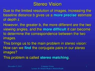
Stereo Vision. Due to the limited resolution of images, increasing the baseline distance b gives us a more precise estimate of depth z.

Stereo Vision
E N D
Presentation Transcript
Stereo Vision • Due to the limited resolution of images, increasing the baseline distance b gives us a more precise estimate of depth z. • However, the greater b, the more different are the two viewing angles, and the more difficult it can become to determine the correspondence between the two images. • This brings us to the main problem in stereo vision: How can we find the conjugate pairs in our stereo images? • This problem is called stereo matching. Computer Vision Lecture 20: Hidden Markov Models/Depth
Stereo Matching • In stereo matching, we have to solve a problem that is still under investigation by many researchers, called the correspondence problem. • It can be phrased like this: • For each point in the left image, find the corresponding point in the right image. • The idea underlying all stereo matching algorithms is that these two points should be similar to each other. • So we need a measure for similarity. • Moreover, we need to find matchable features. Computer Vision Lecture 20: Hidden Markov Models/Depth
Stereo Matching • A straightforward approach to stereo matching uses pyramids , i.e., representations of the two camera images at various resolutions. • The low-resolution versions of two corresponding rows are used to determine the “rough” matching, i.e. large patterns that match between the images. • The precise disparity is determined in the high-resolution images. • As a measure of similarity, we could simply use pieces of a row in the left image as convolution filters and apply them to the corresponding row in the right image. Computer Vision Lecture 20: Hidden Markov Models/Depth
Generating Interesting Points • Using interpolation to determine the depth of points within large homogeneous areas may cause large errors. • To overcome this problem, we can generate additional interesting points that can be matched between the two images. • The idea is to use structured light, i.e., project a pattern of light onto the visual scene. • This creates additional variance in the brightness of pixels and increases the number of interesting points. Computer Vision Lecture 20: Hidden Markov Models/Depth
Generating Interesting Points Computer Vision Lecture 20: Hidden Markov Models/Depth
Shape from Shading • Besides binocular disparity, there are many different ways of depth estimation based on monocular information. • For example, if we know the reflective properties of the surfaces in our scene and the position of the light source, we can use shape from shading techniques: • Basically, since the amount of light reflected by a surface depends on its angle towards the light source, we can estimate the orientation of surfaces based on their intensity. • More sophisticated methods also use the contours of shadows cast by objects to estimate the shape and orientation of those objects. Computer Vision Lecture 20: Hidden Markov Models/Depth
Photometric Stereo • To improve the coarse estimates of orientation derived from shape from shading methods, we can use photometric stereo. • This technique uses three light sources that are located at different, known positions. • Three images are taken, one for each light source, with the other two light sources being turned off. • This way we determine three different intensities for each surface in the scene. • These three values put narrow constraints on the possible orientation of a surface and allow a rather precise estimation. Computer Vision Lecture 20: Hidden Markov Models/Depth
Shape from Texture • As we discussed before, the texture gradient gives us valuable monocular depth information. • At any point in the image showing texture, the texture gradient is a two-dimensional vector pointing towards the steepest increase in the size of texture elements. • The texture gradient across a surface allows a good estimate of the spatial orientation of that surface. • Of course, it is important for this technique that the image has high resolution and a precise method of texture size (granularity) measurement is used. Computer Vision Lecture 20: Hidden Markov Models/Depth
Shape from Motion • The shape from motion technique s similar to binocular stereo, but it uses only one camera. • This camera is moved while it takes images from the visual scene. • This way two images with a specific baseline distance can be obtained, and depth can be computed just like for binocular stereo. • We can even use more than two images in this computation to get more robust measurements of depth. • The disadvantages of shape from motion techniques are the technical overhead for moving the camera and the reduced temporal resolution. Computer Vision Lecture 20: Hidden Markov Models/Depth
Range Imaging • If we can determine the depth of every pixel in an image, we can make this information available in the form of a range image. • A range image has exactly the same size and number of pixels as the original image. • However, each pixel does not specify color or intensity, but the depth of that pixel in the original image, encoded as grayscale. • Usually, the brighter a pixel in a range image is, the closer the corresponding pixel is to the observer. • By providing both the original and the range image, we basically define a 3D image. Computer Vision Lecture 20: Hidden Markov Models/Depth
Sample Range Image of a Mug Computer Vision Lecture 20: Hidden Markov Models/Depth
Range Imaging Through Triangulation • How can we obtain precise depth information for every pixel in the image of a scene? • One precise but slow method uses a laser that can rotate around its vertical axis and can also assume different vertical positions. • This laser systematically and sequentially illuminates points in the image. • A scene camera determines the position of every single point in its picture. • The trick is that this camera looks at the scene from a different direction than does the laser pointer. • Therefore, the depth of every point can be easily and precisely determined through triangulation: Computer Vision Lecture 20: Hidden Markov Models/Depth
Range Imaging Through Triangulation Computer Vision Lecture 20: Hidden Markov Models/Depth
Range Imaging Through Triangulation • Obviously, this is a very slow process and not suitable for dynamic scenes. • To speed things up, we can use a laser that projects a vertical line of light onto the scene. • This laser rotates around its vertical axis and thereby moves the vertical line of light across the scene. • Since only the horizontal positions of points vary and give us depth information, the vertical order of points is preserved. • This allows us to compute the depth of each point along the vertical line without ambiguities. Computer Vision Lecture 20: Hidden Markov Models/Depth
Range Imaging Through Triangulation Computer Vision Lecture 20: Hidden Markov Models/Depth
Range Imaging Through Triangulation • Although this method is faster, it still requires a complete horizontal scan before a depth image is complete. • Maybe we should use a pattern of many vertical lines that only needs to be shifted by the distance between neighboring lines? • The disadvantage of this idea is that we could confuse points in different vertical lines, i.e., associate points with incorrect projection angles. • However, we can overcome this problem by taking multiple images of the same scene with the pattern in the same position. • In each picture, a different subset of lines is projected. Computer Vision Lecture 20: Hidden Markov Models/Depth
Range Imaging Through Triangulation • Then each line can be uniquely identified by its pattern of presence/absence across the images. • For example, for 7 vertical lines we need a series of 3 images to do this encoding: Obviously, with this technique we can encode up to (n – 1) lines using log2(n) images. Therefore, this method is more efficient than the single-line scanning technique. Computer Vision Lecture 20: Hidden Markov Models/Depth
Range Imaging Through Triangulation Computer Vision Lecture 20: Hidden Markov Models/Depth
Now we will talk about…Motion Analysis Computer Vision Lecture 20: Hidden Markov Models/Depth
Motion analysis • Motion analysis is dealing with three main groups of motion-related problems: • Motion detection • Moving object detection and location. • Derivation of 3D object properties. • Motion analysis and object tracking combine two separate but inter-related components: • Localization and representation of the object of interest (target). • Trajectory filtering and data association. • One or the other may be more important based on the nature of the motion application. Computer Vision Lecture 20: Hidden Markov Models/Depth
Motion analysis Computer Vision Lecture 20: Hidden Markov Models/Depth
Differential Motion Analysis • A simple method for motion detection is the subtraction of two or more images in a given image sequence. • Usually, this method results in a difference image d(i, j), in which non-zero values indicate areas with motion. • For given images f1 and f2, d(i, j) can be computed as follows: • d(i, j) = 0 if | f1(i, j) – f2(i, j) | • = 1 otherwise Computer Vision Lecture 20: Hidden Markov Models/Depth
Differential Motion Analysis Computer Vision Lecture 20: Hidden Markov Models/Depth
Difference Pictures Another example of a difference picture that indicates the motion of objects ( = 25). Computer Vision Lecture 20: Hidden Markov Models/Depth
Difference Pictures Applying a size filter (size 10) to remove noise from a difference picture. Computer Vision Lecture 20: Hidden Markov Models/Depth
Difference Pictures The differential method can rather easily be “tricked”. Here, the indicated changes were induced by changes in the illumination instead of object or camera motion (again, = 25). Computer Vision Lecture 20: Hidden Markov Models/Depth
Differential Motion Analysis • In order to determine the direction of motion, we can compute the cumulative difference image for a sequence f1, …, fn of more than two images: Here, f1 is used as the reference image, and the weight coefficients ak can be used to give greater weight to more recent frames and thereby highlight the current object positions. Computer Vision Lecture 20: Hidden Markov Models/Depth
Cumulative Difference Image Example: Sequence of 4 images: a2 = 1 a3 = 2 a4 = 4 Result: Computer Vision Lecture 20: Hidden Markov Models/Depth
Differential Motion Analysis Generally speaking, while differential motion analysis is well-suited for motion detection, it is not ideal for the analysis of motion characteristics. Computer Vision Lecture 20: Hidden Markov Models/Depth