Download
1 / 26
300 likes | 517 Vues
Stereo Vision. Why? Two images provide information to extract (some) 3D information We have good biological models (our own vision system) Difficulties Matching information from left to right … but we’ve already looked at some matching techniques

E N D
Stereo Vision • Why? • Two images provide information to extract (some) 3D information • We have good biological models (our own vision system) • Difficulties • Matching information from left to right • … but we’ve already looked at some matching techniques • … and some can take advantage of expectation • Calibrating the stereo rig • Some methods require careful calibration • Others avoid calibration entirely
Multiple Coordinate Frames • World Frame (Euclidean) • “Arbitrary” origin, z usually vertical • Camera Frame (Euclidean) • Focal point of the camera is the origin, Z points away from the image plane and is aligned with the optical axis. • Image Frame (Euclidean) • Axes X and Y aligned with camera frame. Origin is where the focal ray hits the image plane. • Image Frame (Affine) • Y, Z same as Camera frame, X maybe not perpendicular to Y (models non-rectangular pixels)
Perspective Projection Geometry (review) Y Focal point y 0 f Z Image plane y/f = Y/Z y = fY/Z Z=fY/y
Triangulation • Given image point (x), and focal center (c), all possible world points lie along a ray with vector v: • Find the intersection of these rays to get the 3D point, (see section 7.1 for least-squares formulation) Figure 7.1
Stereo Reconstruction • Epipolar geometry • Every point in one image, lies on a line in the other image • The epipolar line is the image of the ray from the focal point through the point • All epipolar lines pass through the epipole, which is the image of the focal point itself. • So what? • If cameras are calibrated, make epipolar lines line up on scan lines (epipole is at infinity) This is the “canonical configuration”) • If cameras are not calibrated, find the epipole and use it for calibration (8 point algorithm)
Epipolar Geometry Epipolar points (e0 and e1), lines (l0 and l1) and corresponding points (x and x1) Figure 7.3
Epipolar Geometry Definitions • c0, c1 - camera centers of focus • i0, i1 - image planes • p - point in space • x0, x1 – images of p • e0 – epipole 0 (image of c1 in i0) & vice versa for e1 • Epipolar lines l0 and l1 connect e0 and x0; e1 and x1 • Epipolar plane contains p, c0 and c1 (and all epipolar lines) • Epipolar constraint: All images of a point lie on its epipolar line.
Recovering the Epipolar Information • Begin by assuming 2 cameras are related by rotation R and translation T (We will not have to know R and T later) • Then: • (x0, y0, w0)T = P1 (X, Y, Z, 1)T • Where P1 = (Id | 0) and Id is the 3x3 identity matrix • (x1, y1, w1)T = P2 (X, Y, Z, 1)T • Where P2 = (R | -RT)T and R and T are the rotation and translation matrices between the cameras • The image of the line that passes through 2 points (the camera origin C0 = (0, 0, 0, 1) and the point at infinity (x0, y0, z0, 0) is epipolar line 2 • After some algebra (section 7.2), we get the important equation relating the points in the two images: (x0, y0, w0) E (x1, y1, w1)T = 0 E is the 3x3 essential matrix that relates the two images
Recovering the Epipolar Information • The equation (x0, y0, w0) Q (x1, y1, w1)T = 0 is true for every point that is visible in both images! • Since Q is a 3x3 matrix, we would need 9 linear equations to recover all 9 elements • But, we will never be able to recover absolute scale (since moving the camera closer is entirely equivalent to making the objects bigger) • Set Q[3][3] = 1 • Use 8 correspondences to recover 8 points • "8 point algorithm" for epipolar constraint recovery • Given Q and p0 = (x0, y0, s0), the epipolar line is the set of all points P1 for which p0Qp1 = 0, which is an equation for the epipolar line!
Value of Epipolar Information • Recover epipole to use as a constraint for correspondence matching • Use epipolar information to warp images as they would appear in a calibrated rig (epipolar line -> x axis) • Recognize "possible / impossible" relationships among points based on epipolar constraints • Use the concept of "two views" in other ways • Object and shadow • Two copies of the same object (translational symmetry) • Surface of revolution (rotational symmetry of boundary curve)
Stereo in a Calibrated Rig • Assume cameras aligned on x axis, b and f known • Given xl and xr (and d = xl – xr), calculate Z Cl xl = f Xl / Z xr = f Xr / Z = f(Xl – b)/Z xl – xr = (f/Z) (Xl – (Xl – b)) xl – xr = f b / z f xl b f xr Cr P = Xl,Z (left) Xr = Xl – b Zr = Zl = Z
Disparity Image • Given two rectified images (epipolar lines are horizontal or vertical), compute disparity (d) at each point • Disparity image (x, y ,d): x and y from image 0, d is the disparity • Distance is inversely proportional to disparity • Brighter points are closer
Finding Disparities • This is a matching problem • Use knowledge of camera setup to limit match locations • Along horizontal lines, for calibrated setup earlier • Along epipolar lines more generally • Matching strategies include: • Correlation (e.g. random dot stereogram) • (Point) feature extraction & matching • Object recognition & matching [not used by human vision] • Use of relational constraints (items don't trade places)
Sparse vs. Dense Stereo • Feature-based methods are sparse • First, find matchable features, then compute disparities via matches • Less computationally intensive (historically important) • Matches have high certainty • We want dense 3D information • Necessary for modeling, rendering • One way: use sparse matches as seeds, then fill in to make denser maps (analogs: region growing, thresholding with hysteresis)
Dense Stereo Taxonomy • Most methods perform the following steps: • Matching cost computation • Cost (support) aggregation • Disparity computation / optimization • Disparity refinement • “Cost” is generally with respect to an optimization framework (e.g. penalty for non-smoothness)
Sum of Squared Difference (local) • Matching cost is squared difference of intensity at given disparity (i.e. how different are the ‘matching’ pixels?) • Aggregation is adding up cost (at a given disparity) in a square window • Disparity selected based on minimum cost at each pixel • (Optional disparity refinement step can be added)
Optimization Algorithms (global) • Choose a local matching cost (similarity measure) • Apply global constraints (e.g. smoothness) • Use an optimization technique (e.g. simulated annealing, dynamic programming) to solve the resulting constrained optimization problem • Disparity refinement step can be added here
Dynamic Programming for Optimization • Row is left scanline, column is right scanline • Goal: generate least-cost diagonal path through matrix • M=match, L=left only, R=right only (L and R have fixed costs, M depends on match quality)
Disparity Refinement • For rendering, prevent ‘viewmaster’ appearance: • Objects seem to be aligned on fixed planes, e.g. cardboard cutouts stacked behind each other • Interpolate (“subpixel”) disparities to fit appropriate 3D curves and surfaces • Determine areas of occlusion (& verify) • Clean up noise with median filters, etc.
Segmentation Based Approach • First, segment the image into coherent regions • Oversegment to avoid mis-segmentation • Then, fit a local plane to each region • Iterative optimization technique, like relaxation • Allows for arbitrary discontinuities between regions • These techniques are best-ranked on Middlebury stereo evaluation site: • http://vision.middlebury.edu/stereo
Variations on Stereo • Trinocular stereo • Three calibrated cameras impose more constraints on correspondences • Multi-baseline stereo • When b is large, Z determination is more accurate • "error diamonds" are not so elongated • When b is small, correspondences are easier to find • Sliding camera or 3 or more collinaer cameras allow both • (Depth estimate from small b constraints search in larger b)
Motion from 2D Image Sequences • Motion also gives multiple views • Multiple frames of translational motion similar to multiple-baseline images • Correspondence between sequential frames (small baseline) • Reconstruction using first and last frame (large baseline) • Camera moving on known path (e.g. into scene) allows reconstruction of unmoving objects from optical flow • Stable camera, single moving object • Motion segmentation • Trajectory estimation • Possible 3D reconstruction depending on complexity of object and trajectory
Stationary Object, Fixed Background • One or more discrete "moving objects" in the scene • Since most of the scene is stable, image subtraction will highlight objects • What changes are the leading & trailing edges • Changes are of opposite sign • Bounding box of moving object easy to determine • For best results, filter small noise regions • Smoothing before subtraction • Remove small regions of motion after subtraction • Closing to fill small gaps in moving objects' shapes
Optical Flow • Assume that intensity is not changing • Compute vector of each visible point between frames • Set of vectors is "optical flow field" • Issues • Computing point correspondences gives sparse field • Additional constraint from assuming consistent motion • Dense field computed as optimization with correlation and smoothness constraints • When object edges are not visible, only the motion normal to visible edges can be determined (aperture problem). • E.g. looking at a pole through a keyhole
Interpreting Optical Flow Field • Mostly 0, some regions of consistent vector • Translational object motion on stable background • Entire image is consistent vector • Translational camera motion in stable scene • Vectors pointing outward from a point • Motion into the scene towards that point, or expansion • Vectors pointing inward toward a point • Motion away from that point, or contraction • In all cases, larger vectors = faster motion
Range Sensing - Direct 3D • Structured light (visible, infrared, laser) • Simple case: replace second camera by a scanning laser - No correspondence problem! • More efficient: use stripes aligned with rows/columns; use patterns to avoid scanning • Active sensing (radar, sonar, laser, touch?) • Send out a signal & see how long it takes to bounce back • Use phase difference for more accurate data • Act on the object and record results (touch gives position and orientation of surface)