Download

1 / 88
1.11k likes | 2.15k Vues
What Happened Last Time?. Human 3D perception (3D cinema)Computational stereoIntuitive explanation of what is meant by disparityStereo matching problemVarious applications of stereo. What Is Going to Happen Today?. Stereo from a technical point of view:Stereo pipelineEpipolar geometryEpipola

E N D
1. Fundamentals of Stereo Vision Michael Bleyer
LVA Stereo Vision
2. What Happened Last Time? Human 3D perception (3D cinema)
Computational stereo
Intuitive explanation of what is meant by disparity
Stereo matching problem
Various applications of stereo
3. What Is Going to Happen Today? Stereo from a technical point of view:
Stereo pipeline
Epipolar geometry
Epipolar rectification
Depth via triangulation
Challenges in stereo matching
Commonly used assumptions
Middlebury stereo benchmark
4. Michael Bleyer
LVA Stereo Vision
5. Stereo Pipeline
6. Stereo Pipeline
7. Stereo Pipeline
8. Stereo Pipeline
9. Pinhole Camera Simplest model for describing the projection of a 3D scene onto a 2D image.
Model is commonly used in computer vision.
10. Image Formation Process Let us assume we have a pinhole camera.
The pinhole camera is characterized by its focal point Cl and its image plane L.
11. Image Formation Process We also have a second pinhole camera <Cr,R>.
We assume that the camera system is fully calibrated, i.e. the 3D positions of <Cl, L> and <Cr,R> are known.
12. Image Formation Process We have a 3D point P.
13. Image Formation Process We compute the 2D projection pl of P onto the image plane of the left camera L by intersecting the ray from Cl to P with the plane L.
This is what is happening when you take a 2D image of a 3D scene with your camera (image formation process).
14. Image Formation Process We compute the 2D projection pl of P onto the image plane of the left camera L by intersecting the ray from Cl to P with the plane L.
This is what is happening when you take a 2D image of a 3D scene with your camera (image formation process).
15. 3D Reconstruction Task: We have a 2D point pl and want to compute its 3D position P.
16. 3D Reconstruction P has to lie on the ray of Cl to pl.
Problem: It can lie anywhere on this ray.
17. 3D Reconstruction Let us assume we also know the 2D projection pr of P onto the right image plane R.
18. 3D Reconstruction P can now be reconstructed by intersecting the rays Clpl and Crpr.
19. 3D Reconstruction P can now be reconstructed by intersecting the rays Clpl and Crpr.
20. 3D Reconstruction P can now be reconstructed by intersecting the rays Clpl and Crpr.
21. Epipolar Geometry We have stated that P has to lie on the ray Clpl.
22. Epipolar Geometry If we project each candidate 3D point onto the right image plane, we see that the all lie on a line in R.
23. Epipolar Geometry If we project each candidate 3D point onto the right image plane, we see that the all lie on a line in R.
24. Epipolar Geometry If we project each candidate 3D point onto the right image plane, we see that the all lie on a line in R.
25. Epipolar Geometry If we project each candidate 3D point onto the right image plane, we see that the all lie on a line in R.
26. Epipolar Geometry This line is called epipolar line of pl.
This epipolar line is the projection of the ray Clpl onto the right image plane R.
The pixel pr is forced to lie on pl�s epipolar line.
27. Epipolar Geometry This line is called epipolar line of pl.
This epipolar line is the projection of the ray Clpl onto the right image plane R.
The pixel pr is forced to lie on pl�s epipolar line.
28. Epipolar Rectification Specifically interesting case:
Image plane L and R lie in a common plane.
X-axes are parallel to the baseline
Epipolar lines coincide with horizontal scanlines => corresponding pixels have the same y-coordinate
29. Epipolar Rectification Specifically interesting case:
Image plane L and R lie in a common plane.
X-axes are parallel to the baseline
Epipolar lines coincide with horizontal scanlines => corresponding pixels have the same y-coordinate
30. Epipolar Rectification Specifically interesting case:
Image plane L and R lie in a common plane.
X-axes are parallel to the baseline
Epipolar lines coincide with horizontal scanlines => corresponding pixels have the same y-coordinate
31. Epipolar Rectification Specifically interesting case:
Image plane L and R lie in a common plane.
X-axes are parallel to the baseline
Epipolar lines coincide with horizontal scanlines => corresponding pixels have the same y-coordinate
32. Epipolar Rectification Specifically interesting case:
Image plane L and R lie in a common plane.
X-axes are parallel to the baseline
Epipolar lines coincide with horizontal scanlines => corresponding pixels have the same y-coordinate
33. Epipolar Rectification This special case can be achieved by reprojecting left and right images onto virtual cameras.
This process is known as epipolar rectification.
Throughout the rest of the lecture we assume that images have been rectified.
34. Epipolar Constraint � Concluding Remarks Epipolar constraint should always be used, because:
1D search is computationally faster than 2D search.
Reduced search range lowers chance of finding a wrong match (Quality of depth maps).
More or less the only constraint that will always be valid in stereo matching (unless there are calibration errors).
35. Stereo Pipeline
36. Depth via Triangulation
37. Depth via Triangulation
38. Depth via Triangulation
39. Depth via Triangulation
40. Depth via Triangulation
41. Depth via Triangulation
42. Depth via Triangulation
43. Depth via Triangulation
44. Depth via Triangulation From similar triangles:
Write X in explicit form:
Combine both equations:
Write Z in explicit form:
45. Depth via Triangulation From similar triangles:
Write X in explicit form:
Combine both equations:
Write Z in explicit form:
46. Stereo Pipeline
47. Michael Bleyer
LVA Stereo Vision
48. Stereo Matching
49. Why is Stereo Matching Challenging? (1) Color inconsistencies:
When solving the stereo matching problem, we typically assume that corresponding pixels have the same intensity/color (= Photo consistency assumption)
That does not need to be true due to:
Image noise
Different illumination conditions in left and right images
Different sensor characteristics of the two cameras.
Specular reflections (mirroring)
Sampling artefacts
Matting artefacts
50. Why is Stereo Matching Challenging? (2) Untextured regions (Matching ambiguities)
There needs to be a certain amount of intensity/color variation (i.e. texture) so that a pixel can be uniquely matched in the other view.
Can you (as a human) depict depth if you are standing in front of a wall that is completely white?
51. Why is Stereo Matching Challenging? (3) Occlusion Problem
There are pixels that are only visible in exactly one view.
We call this pixels occluded (or half-occluded)
It is difficult to estimate depth for these pixels.
Occlusion problem makes stereo more challenging than a lot of other computer vision problems.
52. The Occlusion Problem Let�s consider a simple scene composed of a foreground and a background object
53. Regular case:
The white pixel P1 can be seen by both camera.
54. Occlusion in the right camera:
The left camera sees the grey pixel P2.
The ray from the right camera to P2 hits the white foreground object => P2 cannot be seen by right camera.
55. Occlusion in the left camera:
The right camera sees the grey pixel P3.
The ray from the left camera to P3 hits the white foreground object => P3 cannot be seen by left camera.
56. Occlusions occur in the proximity of disparity discontinuities.
57. Occlusions occur in the proximity of disparity discontinuities.
58. In the left image, occlusions are located to the left of a disparity boundary.
In the right image, occlusions are located to the right of a disparity boundary.
59. It is difficult to find disparity in the matching point does not exist.
Ignoring the occlusion problem leads to disparity artefacts near disparity borders.
60. It is difficult to find disparity in the matching point does not exist.
Ignoring the occlusion problem leads to disparity artefacts near disparity borders.
61. Michael Bleyer
LVA Stereo Vision
62. Assumptions Assumptions are needed to solve the stereo matching problem.
Stereo methods differ in
What assumptions they use
How they implement these assumptions
We have already learned two assumptions:
Which ones?
63. Photo Consistency and Epipolar Assumptions Photo consistency assumption:
Corresponding pixels have the same intensity/color in both images.
Epipolar assumption:
The matching point of a pixel has to lie on the same horizontal scanline in the other image.
We can combine both assumptions to obtain our first stereo algorithm.
Algorithm 1:
For each pixel p of the left image, search the pixel q in the right image that
lies on the same y-coordinate as p (Epipolar assumption) and
has the most similar color in comparison to p (Photo Consistency).
64. Results of Algorithm 1 Quite disappointing, why?
We have posed the following task:
I have a red pixel. Find me a red pixel in the other image.
Problem:
There are usually many red pixels in the other image (ambiguity)
We need additional assumptions.
65. Results of Algorithm 1 What is the most obvious difference between the correct and the computed disparity maps?
66. Smoothness Assumption (1) Observation:
A correct disparity map typically consists of regions of constant (or very similar) disparity. For example, lamp, head, table,�
We can give this apriori knowledge to a stereo algorithm in the form of a smoothness assumption
67. Smoothness Assumption (2) Smoothness assumption:
Spatially close pixels have the same (or similar) disparity.
(By spatially close I mean pixels of similar image coordinates.)
Smoothness assumption typically holds true almost everywhere, except at disparity borders.
68. Smoothness Assumption (3) Almost every stereo algorithm uses the smoothness assumption.
Stereo algorithms are commonly divided into two categories based on the form in which they apply the smoothness assumption.
These categories are:
Local methods
Global methods
69. Local Methods Compare small windows in left and right images.
Within the window, pixels are supposed to have the same disparity => implicit smoothness assumption.
We will learn a lot about them in the next session.
70. Global Methods Define a cost function to measure the quality of a disparity map:
High costs mean that the disparity map is bad.
Low costs mean it is good.
Costs function is typically in the form of:
where
Edata measures photo consistency
Esmooth measures smoothness
Global methods express smoothness assumption in an explicit form (as a smoothness term).
The challenge is to find a disparity map of minimum costs (sessions 4 and 5).
71. Uniqueness Constraint The uniqueness constraint will help us to handle the occlusion problem.
It states:
A pixel in one frame has at most a single matching point in the other frame.
In general valid, but broken for:
Transparent objects
Slanted surfaces
72. Uniqueness Constraint
73. Uniqueness Constraint
74. Uniqueness Constraint
75. Uniqueness Constraint
76. Other Assumptions Ordering assumption:
The order in which pixels occur is preserved in both images.
Does not hold for thin foreground object.
Disparity gradient limit:
Originates from psychology
Not clear whether assumption is valid for arbitrary camera setups.
Both assumptions have rarely been used recently => they are slightly obsolete.
77. Michael Bleyer
LVA Stereo Vision
78. Ground Truth Data Ground truth = the correct solution to a given problem.
The absence of ground truth data has represented a major problem in computer vision:
For most computer vision problems, not a single �real� test image with ground truth solution has been available.
Computer-generated ground truth images do oftentimes not reflect the challenges of real data recorded with a camera.
It is difficult to measure the progress in a field if there is no commonly agreed data set with ground truth solution.
79. Ground Truth Data Ground Truth data is now available for a wide range of computer vision problems including:
Object recognition
Alpha matting
Optical flow
MRF-optimization
Multi view reconstruction
�
For stereo, ground truth data is available on the Middlebury Stereo Evaluation website http://vision.middlebury.edu/stereo/
The Middlebury set is widely adopted in the stereo community.
80. The Middlebury Set
81. How Can One Generate Ground Truth Disparities? Hand labelling:
Tsukuba test set
Extremely labor-intensive
Most other Middlebury ground truth disparity maps have been created using a more precise depth computation technique than stereo matching, namely structured light.
82. Setup Used for Generating the Middlebury Images Different light patterns are projected onto the scene to compute a high-quality depth map (Depth from structured light).
83. Setup Used for Generating the Middlebury Images Different light patterns are projected onto the scene to compute a high-quality depth map (Depth from structured light).
84. Disparity Map Quality Evaluation in the Middlebury Benchmark Estimation of wrong pixels:
Build absolute difference between computed and ground truth disparity maps.
If absolute disparity difference is larger than one pixel, pixel is counted as error.
3 Error metrics:
Percentage of erroneous pixels in (1) unoccluded regions, (2) the whole image and (3) in regions close to disparity borders.
85. The Middlebury Online Benchmark If you have implemented a stereo algorithm, you can evaluate its performance using the Middlebury benchmark.
You have to run it on these 4 image pairs:
The 3 error metrics are then computed for each image pair.
Your algorithm is then ranked according to the computed error values.
86. The Middlebury Table Currently, more than 70 methods evaluated.
You should use this table to rank your stereo matching algorithm developed as your home work.
87. General Findings in the Middlebury Table Global methods outperform local methods.
Local methods:
Adaptive weight methods represent the state-of-the-art.
Global methods:
Methods that apply Belief Propagation or Graph-Cuts in the optimization step outperform dynamic programming methods (if such categorization makes sense)
All top-performing methods apply color segmentation.
88. Summary 3D geometry
Challenges
Ambiguity
Occlusions
Assumptions
Photo consistency
Smoothness assumption
Uniqueness assumption
Middlebury benchmark